Extra Credit 7

LAST TIME

Build up to Schrödinger Equation: some wonderful surprises

• operators
• eigenvalue equations
• operators in quantum mechanics – especially \(\hat{x} = x\) and \(\hat{p_x} = -i \hbar \frac{\partial}{\partial x}\)
• non-commutation of \(\hat{x}\) and \(\hat{p_x}\) : related to the uncertainty principle
• wavefunctions: probability amplitude, continuous! therefore no perfect localization at a point in space
• expectation value (and normalization)
• \( \hat{H} \Psi = E \Psi\)
• Free Particle
• Particle in 1-D Box (first viewing)

---

Today:

1. Review of Free Particle

some simple integrals

2. Review of Particle in 1-D “Infinite” Box

boundary conditions

pictures of \(\Psi_n(x)\), Memorable Qualitative features

3. Crude uncertainties, \(\Delta x\) and \(\Delta p\), for Particle in Box

4. 3-D Box
separation of variables

Form of \(E_ {n_x,n_y,n_z}\) and \(\Psi_ {n_x,n_y,n_z}\)

---

1. Review of Free Particle: \(V(x) = V_0\)

\(\Psi_ {|k|}(x) = ae^{+ikx} + be^{-ikx}\) complex oscillatory (because \(E < V_0\) )

\(E_k = \frac{{(\hbar k)}^2}{2m} + V_0\) k is not quantized

\(\int_{-\infty}^{\infty}|\Psi_ {|k|}(x)|^2 dx =\int_{-\infty}^{\infty}[{|a|^2}+{|b|^2}+(a^*be^{-ikx}+ab^*e^{ikx})] dx \)

\(={|a|^2} {\infty}+{|b|^2} {\infty}+a^*b0+ab^*0\) (Note what happens to the product \(e^{-ikx}e^{+ikx}\))

can’t normalize \(\Psi=ae^{ikx}\) to 1.

\(\int_{-\infty}^{\infty} dx {|a|^2}e^{-ikx}e^{+ikx} = \int_{-\infty}^{\infty} dx {|a|^2}\)

which blows up. Instead, normalize to specified # of particles between x1 and x2.

---

Questions:

Is \(\Psi_ {|k|}(x) = ae^{+ikx} + be^{-ikx}\) an eigenfunction of \(\hat{p_x}\) ? \(\hat{(p^2)_x}\) ? What do your answers mean? Is \(e^{+ikx}\) eigenfunction of \(\hat{p_x}\) ? What eigenvalue?

---

2. Review of Particle in 1-D Box of length a, with infinitely high walls

“infinite box” or “PIB”

In view of its importance in starting you out thinking about quantum mechanical particle in a well problems, I will work through this problem again, carefully.

\(V(x) = 0\) \(0 ≤ x ≤ a\)

\(V(x) = {\infty}\) \(x<0, x>a\)

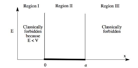
Consider regions I and III.

\(E<V(x)\)

\[\hat{H} = -\frac{\hbar}{2m} \frac{d^2}{dx^2} + {\infty}\]

\[\frac{\hbar}{2m} \frac{d^2}{dx^2} \Psi = ({\infty}-E) \Psi\]

(no matter what finite value we choose for E, the Schrödinger equation can only be satisfied by setting \(\Psi(x) = 0\) throughout regions I and III.)

So we know that \(\Psi(x) = 0\) \(x<0, x>a\)

but \(\Psi(x)\)must be continuous everywhere, thus\(\Psi(0)=\Psi(a) = 0\). These are boundary conditions.

Note, however, that for finite barrier height and width, we will eventually see that it is possible for \(\Psi(x)\) to be nonzero in a classically forbidden \(E<V(x)\) region. “Tunneling.” (There will be a problem on Problem Set #3 about this.)

So we solve for \(\Psi(x)\) in Region II, which looks exactly like the free particle because \(V(x) = 0\) in Region II. Free particle solution are written in sin, \(cos\) form rather than \(e^{-ikx}\) form, because application of boundary conditions is simpler. [This is an example of finding a general principle and then trying to find a way to violate it.]

\(\Psi (x) = Asin kx + Bcos kx\)

Apply boundary conditions

\(\Psi (0) = 0 = 0+B → B=0\)

\(\Psi (a) = 0 =Asin ka ⇒ ka = n\pi\), \(k = \frac{n \pi}{a} \)

Normalize: \[1=\int_{-\infty}^{\infty} dx \Psi^* \Psi = A^2 \int_{0}^{a} dx sin^2 \frac{n \pi}{a} x\]

→ \(A = \left(\frac{2}{a} \right)^\frac{1}{2}\) (Picture of normalization integrand suggests that the value of the normalization integral \(=\frac{a}{2}\))

---

Non-Lecture

Normalization integral for particle-in-a-box eigenfunctions

\(\Psi_n(x) = Asin \frac{n \pi}{a}x\)

Normalization (one particle in the box) requires \(\int_{-\infty}^{\infty} dx \Psi^*\Psi = 1 \).

For\(V(x) = 0\), \(0 ≤ x ≤ a\) infinite wall box:

\[1=\int_{-\infty}^{0} dx \Psi^*\Psi+\int_{0}^{a} dx \Psi^*\Psi+\int_{a}^{\infty} dx \Psi^*\Psi = 0 + {|A|^2} \int_{0}^{a} dx {sin^2}\frac{n \pi}{a}x + 0\]

\(1=|A|^2 \int_{0}^{a} dx sin^2 \frac{n \pi}{a} x\)

Definite integral

\[\int_{0}^{ \pi} dy {sin^2}y=\frac{\pi}{2}\]

change variable: \[y=\frac{n \pi}{a}x\] \[ dy =\frac{n \pi}{a} dx \] \[dx =\frac{a}{n \pi} dy \]

limits of integration:

\[ x=0 ⇒ y=0\]

\[ x=a ⇒ y={n \pi}\]

\[ \int_{0}^{a} dx {sin^2}\frac{n \pi}{a}x = \int_{0}^{n \pi} (\frac{a}{n \pi} ) dy {sin^2}y = \frac{a}{n \pi}n (\frac{\pi}{2}) = \frac{q}{2}\]

\(1=|A|^2 \frac{a}{2} \), Thus \(A = \left(\frac{2}{a} \right)^\frac{1}{2}\)

\(\Psi_n(x) = Asin \frac{n \pi}{a}x\) (A very good equation to remember! )

End of Non-Lecture

---

Find \(E_n\). These are all of the allowed energy levels.

\( \hat{H} \Psi_n = E_n \Psi_n\)

\[-\frac{\hbar^2}{2m} \frac{d^2}{dx^2} \Psi_n = E_n \Psi_n\]

\[-\frac{\hbar^2}{2m} {(k_n)^2}=E_n=\frac{h^2}{4 \Pi^2} \frac{1}{2m} \frac{n^2 \Pi^2}{a^2} = n^2(\frac{h^2}{8ma^2} )\]

\[(k_n)^2=\frac{n^2 \Pi^2}{a^2}, (\frac{h^2}{8ma^2} )=E_1\]

\[n=1, 2, …\]

n = 0 would correspond to empty box

Energy levels are integer multiples of a common factor, \[E_n=E_1n^2\]. (This will turn out to be of special significance when we look at solutions of the time-dependent Schrödinger equation (Lecture #13).

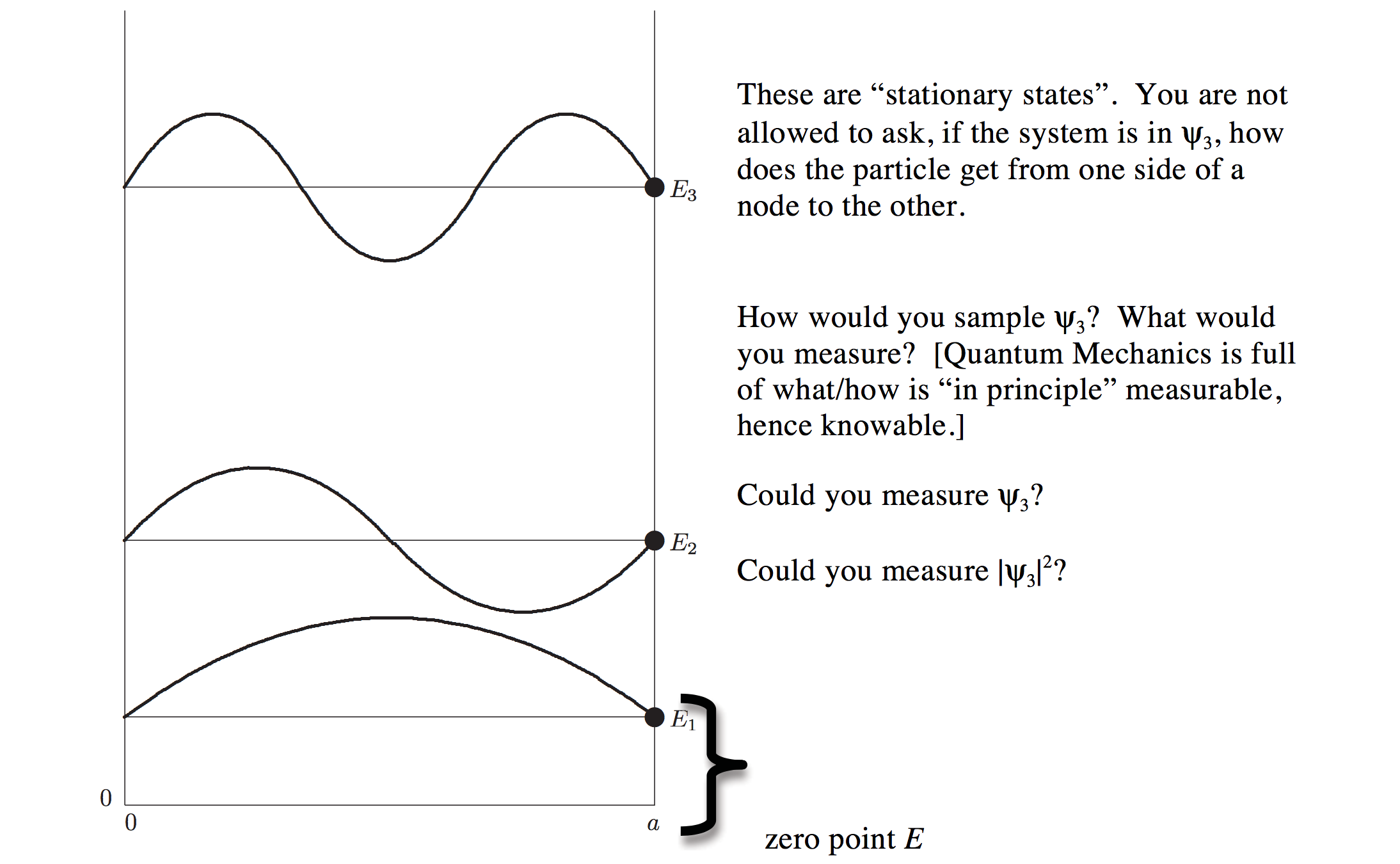
All bound systems have their lowest energy level at an energy greater than the energy of the bottom of the well: “zero-point energy”

This zero-point energy is a manifestation of the uncertainty principle. Why? What is the momentum of a state with zero kinetic energy? Is this momentum perfectly specified? What does that require about position?

---

3. Crude estimates of \(\Delta x \Delta p\)

(we will make a more precise definition of uncertainty in the next lecture)

\(\Delta x = a\) for all n (the width of the well)

\(\Delta p_n = +\hbar k_n-(-\hbar k_n) = 2\hbar |k_n|=2\hbar \frac{n \pi}{a}\)

\(=\frac{2}{2 \pi}h\frac{n \pi}{a}=h\frac{n}{a}\)

The joint uncertainty is

\(\Delta x_n \Delta p_n=(a)\frac{nh}{a}=hn\) which increases linearly with n.

n = 0 would imply \(\Delta p_n=0\) and the uncertainty principle would then require \(\Delta x_n={\infty}\) , which is impossible! This is an indirect reason for the existence of zero-point energy.

Since the uncertainty principle is \(\Delta x \Delta p = h\)

it appears that the n = 1 state is a minimum uncertainty state. It will be generally true that the lowest energy state in a well is a minimum uncertainty state.

---

4. Use the 3-D box to illustrate a very convenient general result: separation of variables.

Whenever it is possible to write \(\hat{H}\) in the form:

\(\hat{H}=\hat{h_x}+\hat{h_y}+\hat{h_z}\) (provided that the additive terms are mutually commuting)

\(\hat{p_x}^2+V_x(\hat{x})+etc\).

it is possible to obtain ψ and E in separated form (which is exceptionally convenient!):

\(\Psi(x, y, z )= \Psi_x(x)\Psi_y(y)\Psi_z(z)\)

\(E=E_x+E_y+E_z\).

Or, more generally, when

\(\hat{H}=\sum_{i=1}^{n} \hat{h_i}(q_i)\)

then \(\Psi=\sum_{i=1}^{n} \Psi_i(q_i)

\(E=\sum_{i=1}^{n} E_i\)

Consider the specific example of the 3-D box with edge lengths a, b, and c.

\(V(x, y, z)=0\), \(0 ≤ x ≤ a, 0 ≤ y ≤ b, 0 ≤ z ≤ c\), otherwise \(V={\infty}\).

This is a special case of \(V(x, y, z)=V_x+V_y+V_z\).

\(T(\hat{p_x}+\hat{p_y}+\hat{p_z}) =-\frac{\hbar^2}{2m} [\dfrac {\partial^2}{\partial x^2}+\dfrac {\partial^2}{\partial y^2}+\dfrac {\partial^2}{\partial z^2}]\)

\(\hat{H}(x, y, z) = [-\frac{\hbar^2}{2m} \dfrac {\partial^2}{\partial x^2}+V_x(\hat{x})]+ [-\frac{\hbar^2}{2m} \dfrac {\partial^2}{\partial y^2}+V_y(\hat{y})]+ [-\frac{\hbar^2}{2m} \dfrac {\partial^2}{\partial z^2}V_z(\hat{z})]\)

\(=\hat{h_x}+\hat{h_y}+\hat{h_z}\)

Schrödinger Equation

\([\hat{h_x}+\hat{h_y}+\hat{h_z}]\Psi(x, y, z) = E\Psi(x, y, z)\)

Try \(\Psi(x, y, z) = \Psi_x(x) \Psi_y(y) \Psi_z(z)\),

Where \(\hat{h_i}\) operates only on \(\Psi_i\),

and \(\hat{h_i}\Psi_i=E_i\Psi_i\) are the solutions of the 1-D problem.

\(\hat{h_x}\Psi(x, y, z) = \Psi_y\Psi_z\hat{h_x}\Psi_x=\Psi_y\Psi_zE_x\Psi_x=E_x\Psi_x\Psi_y\Psi_z=E_x\Psi(x, y, z)\).

(does not operate on y, z)

\(\hat{h_y}\Psi=E_y\Psi_x\Psi_y\Psi_z\)

\(\hat{h_z}\Psi=E_z\Psi_x\Psi_y\Psi_z\)

\(\hat{h_x}\Psi+\hat{h_y}\Psi+\hat{h_z}\Psi=\hat{H}\Psi=(E_x+E_y+E_z)\Psi\).

So we have shown that, if \(\hat{H}\) is separable into additive (commuting) terms, then \(\Psi\) can be written as a product of independent factors, and E will be a sum of separate subsystem energies. Convenient!

So, for the a, b, c box \[\Psi_{n_x} =\left(\frac{2}{a} \right)^\frac{1}{2} sin\frac{n_x \pi}{a}\]

\[E_{n_x} =(n_x)^2\frac{h^2}{8ma^2}\]

\[\int_{0}^{a} dx (\Psi_{n_x})^2=1\]

\[\Psi_{n_y} =\left(\frac{2}{b} \right)^\frac{1}{2} sin\frac{n_y \pi}{b}\]

normalized \[E_{n_y} =(n_y)^2\frac{h^2}{8mb^2}\]

\[\Psi_{n_z} =\left(\frac{2}{c} \right)^\frac{1}{2} sin\frac{n_z \pi}{c}\]

normalized \[E_{n_z} =(n_z)^2\frac{h^2}{8mc^2}\]

\[E_{n_x,n_y,x_z} = \dfrac{h^{2}}{8m}\left(\dfrac{n_{x}^{2}}{a^{2}} + \dfrac{n_{y}^{2}}{b^{2}} + \dfrac{n_{z}^{2}}{c^{2}}\right)\]

\[\Psi_{n_x,n_y,x_z} =\left(\frac{8}{abc} \right)^\frac{1}{2} sin\frac{n_x \pi}{z} sin\frac{n_y \pi}{b} sin\frac{n_z \pi}{c}\]

If each of the factors of \[\Psi_{n_x,n_y,x_z}\] is normalized, it’ s easy to show that

\[\int dx dy dz |\Psi_{n_x,n_y,x_z}|^2=1\]

because each of the integrations acts on only one separable factor.

This looks like a lot of algebra, but it really is an important, convenient, and frequently encountered simplification.

We use this separable form for \(\Psi\) and E all of the time, even when \(\hat{H}\)is not exactly separable (for example, a box with slightly rounded corners).

\[\hat{H} = \hat{H}^0 + \hat{H}^1\]

\(\hat{H}\)— a separable Hamiltonian that we use to define a complete set of "basis functions" and "zero-order energyies."

\(\hat{H}^1\) — a correction term that contains what we would like to leave out.

This is the basis for our intuition, names of things, and approximate energy level formulas.

\(\hat{H}^1\)contains small inter-sub-system coupling terms that are dealt with by perturbation

theory (Lectures #15, #16 and #19).

---

NEXT TIME

we are going to look at some properties of a particle in a box. Some of these properties are based on simple insights, while others are based on actually evaluating the necessary integrals.

\[<x>\]

\[<x^2>\]

"variance" \[{\sigma _x}^2=<x^2>-<x>\]

\[<p>\]

\[<x^2>\]

\[\sigma _{p_x}\]

\[{\sigma _x} \sigma _{p_x}\]

FWHM

Gaussian \[G(x-x_0, \sigma _x)\] (\(x_0\) is "center", \(\sigma _x\) is "width")

Lorentzian \[L(x-x_0, \sigma _x)\]

Minimum Uncertainty Wavepacket