Extra Credit 32: Using Gaussian on Athena

First, you need to set up the Gaussian environment, by typing:

athena% setup gaussian

This will take several seconds to run and then a window will pop up with a different prompt:

gaussian%

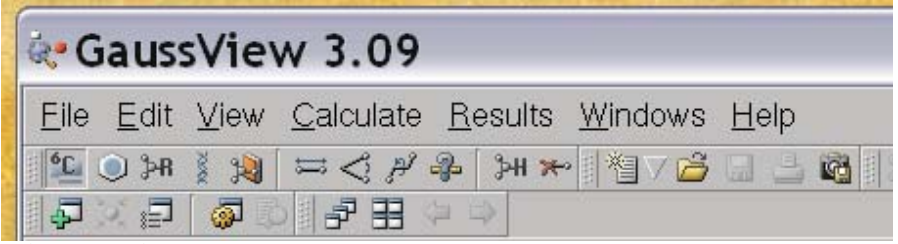
We are going to use the GaussView GUI for the program to run all our calculations, so we type:

gaussian% gv

This will pop up two windows. One is the control window while the other is the molecule window, which should be blank to begin with. For example, it may look like:

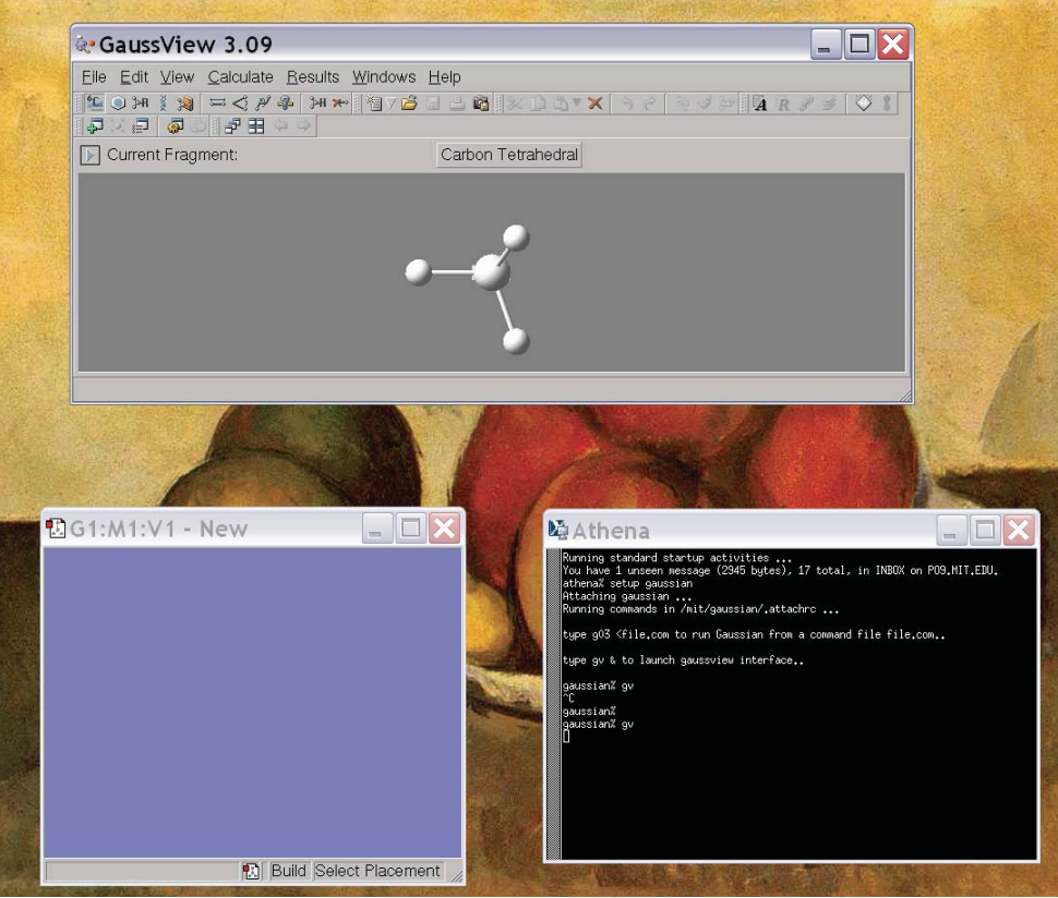
The top window is the control window and the lower left window is the molecule window. Now, our first goal is to create the molecule we are interested in. Generally, there are 4 icons in the control window that are useful for this:

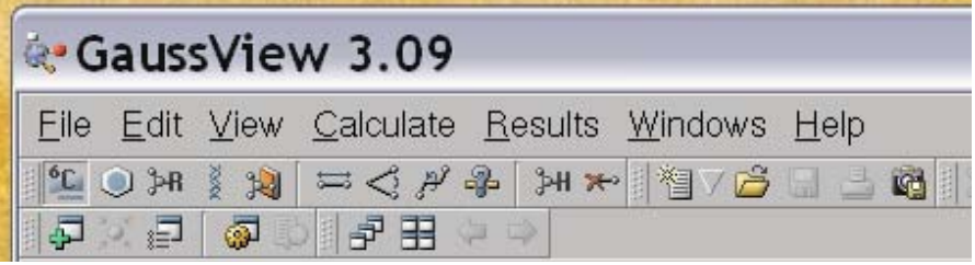
The useful icons for structure building are the first four. Basically the first icon allows you to place an atom, the second allows you to place a few predefined fragments like benzene, pyridine, etc., the second allows you to create some standard R-groups and the fourth allows you to create some biochemical molecules, like amino acids and DNA base pairs. Upon selecting the type of fragment you are interested in, you also have to choose which specific fragment you want. For example, when you select an atom (first icon) it defaults to an sp3 carbon atom:

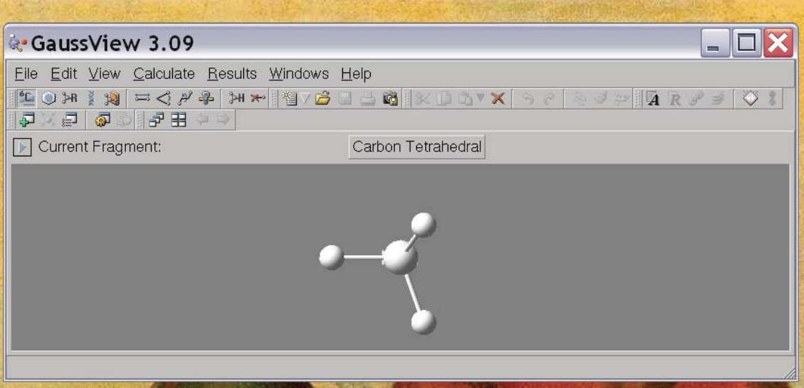
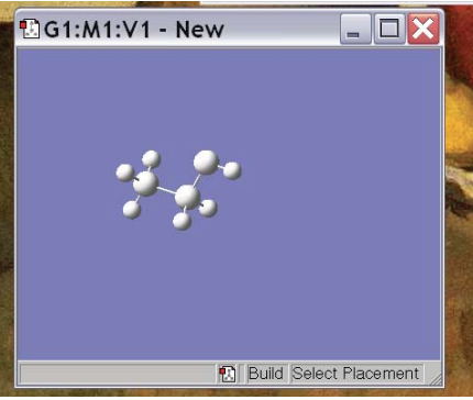
In order to change this, click on “Carbon Tetrahedral” and it will give you all the choices on the periodic table. Once you’ve selected your favorite atom, you can place that atom in your molecule by clicking in the molecule window. For example, if you choose an sp3 nitrogen and click in the molecule window you get the picture at right. Going through a little bit of trial and error, you can then get it to make something interesting, like Ethanol (below). Note that you can re-orient the molecule to get a better perspective by clicking on the molecule and dragging the pointer.

Now, we would like to do some calculations on this molecule. To do this, we click on the “Calculate→Gaussian” tab in the control window. This will pop up yet another window that controls the Gaussian calculation parameters:

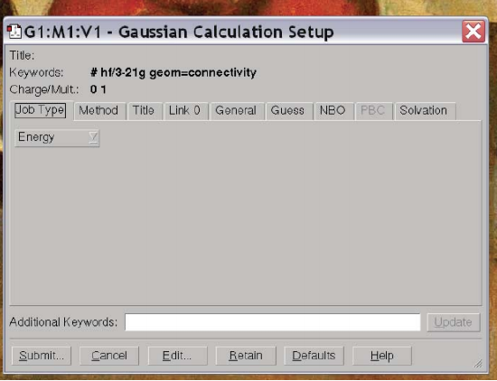
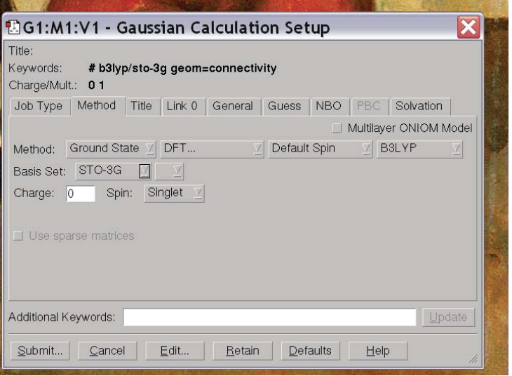
You’ll note that the default is to do a HF/3-21G calculation and compute the energy. We can change all of these options using the tabs. If we click on the button the reads “Energy” we find a bunch of different options for calculations – “Energy”, “Optimize”, “Opt+Freq”, “NMR”, “BOMD”…. These specify different operations you might want Gaussian to perform: compute the energy for the given structure (Energy), compute the optimal structure (Optimize) get the optimal structure and compute vibrational frequencies (Opt+Freq) compute NMR parameters (NMR), perform molecular dynamics (BOMD) …. For now, let’s do an optimization. But let’s say we want to change the method and basis set so that we do a B3LYP calculation in a STO-3G basis. We tab over to Methods and change the method and basis set until it reads as we would like:

At this point, we’re ready to run our calculation, so we click “Submit” in the lower left hand corner. It prompts us if we want to save an input, and we click “Save” and specify a file name for the input. By convention input files end in “.com” so we specify “ethanol.com”. It then prompts us if we want to submit the input file and we click “OK.” The calculation then runs (which will take a minute or so) and Gaussian notifies us that the job is complete. You should then open the output file “ethanol.chk” to view the results.

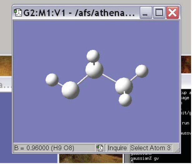
Once the job is done, we can do a few things. First, we can look at the geometry that our optimization produced. To do this we use the next few icons on in the control window:

The 6th, 7th and 8th icons allow you to modify the bond lengths, bond angles and torsion angles in the molecule and the 9th allows you to measure the lengths and angles. To measure, just click on the icon and then click on the atoms that are involved in the distance/angle you are interested in. The measurement will show up in the lower left hand corner of the molecule window. The bottom is an example where we’ve measured a C-H bond distance and it turns out to be .96 Å:

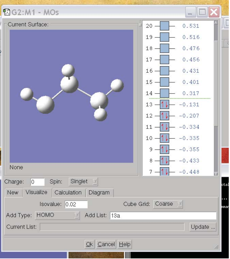
Another thing we are likely to want to do is look at orbitals. To do this, we use the icon on the upper right of the control window that looks like a pz orbital. This will pop up a window that will allow you to make isosurface plots of the various obitals (below). To visualize the orbitals, click on the “visualize” tab. Here, you can specify a grid size (“fine” is usually best) and an isovalue (something around .1 gives reasonable sized orbitals). Further, you can select the orbitals you are interested in by clicking on them in the MO 5.61 Physical Chemistry Lecture 31 5 diagram. Once you have specified the information, click “Update” and a plot of the MO you selected will appear in the MO window.

The final thing we are likely to want to do is to see the energy of the optimized structure. To do this, navigate over to the Results tab and click on Summary. This will pop up a window that has the total energy of the molecule in the present conformation, as well as some additional information including the molecular dipole moment. If you want to compare the stability of two different conformations of a molecule, or two different charge or spin states, you only need to compare the energies of the two species as stated here. I should also note that, after an optimization, the energy displayed is the optimized energy, not the starting energy. That is the bare bones summary of how to use Guassian, covering only the basic features. To learn more about what Gaussian can do, you can take a look at their on-line help manual:

http://www.gaussian.com/g_ur/g03mantop.htm

Happy Computing!