
8: Extra Credit
- Page ID
- 94075
\( \newcommand{\vecs}[1]{\overset { \scriptstyle \rightharpoonup} {\mathbf{#1}} } \)
\( \newcommand{\vecd}[1]{\overset{-\!-\!\rightharpoonup}{\vphantom{a}\smash {#1}}} \)
\( \newcommand{\dsum}{\displaystyle\sum\limits} \)
\( \newcommand{\dint}{\displaystyle\int\limits} \)
\( \newcommand{\dlim}{\displaystyle\lim\limits} \)
\( \newcommand{\id}{\mathrm{id}}\) \( \newcommand{\Span}{\mathrm{span}}\)
( \newcommand{\kernel}{\mathrm{null}\,}\) \( \newcommand{\range}{\mathrm{range}\,}\)
\( \newcommand{\RealPart}{\mathrm{Re}}\) \( \newcommand{\ImaginaryPart}{\mathrm{Im}}\)
\( \newcommand{\Argument}{\mathrm{Arg}}\) \( \newcommand{\norm}[1]{\| #1 \|}\)
\( \newcommand{\inner}[2]{\langle #1, #2 \rangle}\)
\( \newcommand{\Span}{\mathrm{span}}\)
\( \newcommand{\id}{\mathrm{id}}\)
\( \newcommand{\Span}{\mathrm{span}}\)
\( \newcommand{\kernel}{\mathrm{null}\,}\)
\( \newcommand{\range}{\mathrm{range}\,}\)
\( \newcommand{\RealPart}{\mathrm{Re}}\)
\( \newcommand{\ImaginaryPart}{\mathrm{Im}}\)
\( \newcommand{\Argument}{\mathrm{Arg}}\)
\( \newcommand{\norm}[1]{\| #1 \|}\)
\( \newcommand{\inner}[2]{\langle #1, #2 \rangle}\)
\( \newcommand{\Span}{\mathrm{span}}\) \( \newcommand{\AA}{\unicode[.8,0]{x212B}}\)
\( \newcommand{\vectorA}[1]{\vec{#1}} % arrow\)
\( \newcommand{\vectorAt}[1]{\vec{\text{#1}}} % arrow\)
\( \newcommand{\vectorB}[1]{\overset { \scriptstyle \rightharpoonup} {\mathbf{#1}} } \)
\( \newcommand{\vectorC}[1]{\textbf{#1}} \)
\( \newcommand{\vectorD}[1]{\overrightarrow{#1}} \)
\( \newcommand{\vectorDt}[1]{\overrightarrow{\text{#1}}} \)
\( \newcommand{\vectE}[1]{\overset{-\!-\!\rightharpoonup}{\vphantom{a}\smash{\mathbf {#1}}}} \)
\( \newcommand{\vecs}[1]{\overset { \scriptstyle \rightharpoonup} {\mathbf{#1}} } \)
\(\newcommand{\longvect}{\overrightarrow}\)
\( \newcommand{\vecd}[1]{\overset{-\!-\!\rightharpoonup}{\vphantom{a}\smash {#1}}} \)
\(\newcommand{\avec}{\mathbf a}\) \(\newcommand{\bvec}{\mathbf b}\) \(\newcommand{\cvec}{\mathbf c}\) \(\newcommand{\dvec}{\mathbf d}\) \(\newcommand{\dtil}{\widetilde{\mathbf d}}\) \(\newcommand{\evec}{\mathbf e}\) \(\newcommand{\fvec}{\mathbf f}\) \(\newcommand{\nvec}{\mathbf n}\) \(\newcommand{\pvec}{\mathbf p}\) \(\newcommand{\qvec}{\mathbf q}\) \(\newcommand{\svec}{\mathbf s}\) \(\newcommand{\tvec}{\mathbf t}\) \(\newcommand{\uvec}{\mathbf u}\) \(\newcommand{\vvec}{\mathbf v}\) \(\newcommand{\wvec}{\mathbf w}\) \(\newcommand{\xvec}{\mathbf x}\) \(\newcommand{\yvec}{\mathbf y}\) \(\newcommand{\zvec}{\mathbf z}\) \(\newcommand{\rvec}{\mathbf r}\) \(\newcommand{\mvec}{\mathbf m}\) \(\newcommand{\zerovec}{\mathbf 0}\) \(\newcommand{\onevec}{\mathbf 1}\) \(\newcommand{\real}{\mathbb R}\) \(\newcommand{\twovec}[2]{\left[\begin{array}{r}#1 \\ #2 \end{array}\right]}\) \(\newcommand{\ctwovec}[2]{\left[\begin{array}{c}#1 \\ #2 \end{array}\right]}\) \(\newcommand{\threevec}[3]{\left[\begin{array}{r}#1 \\ #2 \\ #3 \end{array}\right]}\) \(\newcommand{\cthreevec}[3]{\left[\begin{array}{c}#1 \\ #2 \\ #3 \end{array}\right]}\) \(\newcommand{\fourvec}[4]{\left[\begin{array}{r}#1 \\ #2 \\ #3 \\ #4 \end{array}\right]}\) \(\newcommand{\cfourvec}[4]{\left[\begin{array}{c}#1 \\ #2 \\ #3 \\ #4 \end{array}\right]}\) \(\newcommand{\fivevec}[5]{\left[\begin{array}{r}#1 \\ #2 \\ #3 \\ #4 \\ #5 \\ \end{array}\right]}\) \(\newcommand{\cfivevec}[5]{\left[\begin{array}{c}#1 \\ #2 \\ #3 \\ #4 \\ #5 \\ \end{array}\right]}\) \(\newcommand{\mattwo}[4]{\left[\begin{array}{rr}#1 \amp #2 \\ #3 \amp #4 \\ \end{array}\right]}\) \(\newcommand{\laspan}[1]{\text{Span}\{#1\}}\) \(\newcommand{\bcal}{\cal B}\) \(\newcommand{\ccal}{\cal C}\) \(\newcommand{\scal}{\cal S}\) \(\newcommand{\wcal}{\cal W}\) \(\newcommand{\ecal}{\cal E}\) \(\newcommand{\coords}[2]{\left\{#1\right\}_{#2}}\) \(\newcommand{\gray}[1]{\color{gray}{#1}}\) \(\newcommand{\lgray}[1]{\color{lightgray}{#1}}\) \(\newcommand{\rank}{\operatorname{rank}}\) \(\newcommand{\row}{\text{Row}}\) \(\newcommand{\col}{\text{Col}}\) \(\renewcommand{\row}{\text{Row}}\) \(\newcommand{\nul}{\text{Nul}}\) \(\newcommand{\var}{\text{Var}}\) \(\newcommand{\corr}{\text{corr}}\) \(\newcommand{\len}[1]{\left|#1\right|}\) \(\newcommand{\bbar}{\overline{\bvec}}\) \(\newcommand{\bhat}{\widehat{\bvec}}\) \(\newcommand{\bperp}{\bvec^\perp}\) \(\newcommand{\xhat}{\widehat{\xvec}}\) \(\newcommand{\vhat}{\widehat{\vvec}}\) \(\newcommand{\uhat}{\widehat{\uvec}}\) \(\newcommand{\what}{\widehat{\wvec}}\) \(\newcommand{\Sighat}{\widehat{\Sigma}}\) \(\newcommand{\lt}{<}\) \(\newcommand{\gt}{>}\) \(\newcommand{\amp}{&}\) \(\definecolor{fillinmathshade}{gray}{0.9}\)Last Time
- What was surprising about Quantum Mechanics?
- Free particle (almost exact reprise of 1D Wave Equation)
- Can't be normalized to 1 over all spaces! Instead: Normalize to one particle between \({x_1}\) and \({x_2}\). What do we mean by "square integrable?"
\[\langle p \rangle = \frac{\lvert a \rvert^2 - |b|^2}{|a|^2+|b|^2}\]
- What does this mean in a click-click experiment?
- Motion not present, but \(\Psi\) is encoded for it.
- Nodes spacing: \(\lambda/2\) (generalize this to get the "semiclassical")
- semiclassical : \(\lambda (x) = \frac{h}{p(x)}\), \(P_{classical}(x) = [2m(E - V(x))]^{1/2}\)
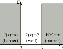
Particle in an Infinite Box
\[E_{n} = \frac{h^2}{8ma^2}n^2\]
\[\Psi_{n}(x) = \left(\frac{2}{a}\right)^{1/2} \sin \left(\frac{n\pi}{a}\right)x\]
(nodes, zero-point energy change: \(a , V_{0}\), locations of left edge
importance of pictures)
3D Box
\[\hat{H} = \hat{h}_x + \hat{h}_y + \hat{h}_z\]
(commuting operators)
\[E_{n_{x}n_{y}n_{z}} = E_{n_{x}}+ E_{n_{y}}+ E_{n_{z}}\]
\[\Psi_{n_{x}n_{y}n_{z}} = \Psi_{n_{x}}(X)\Psi_{n_{y}}(Y)\Psi_{n_{z}}(Z)\]
Today (and Next 3+ Lectures) Harmonic Oscillator
- Classical Mechanics ("normal modes"" of vibration in polyatomic molecules arise from classical mechanics). Preparation for Quantum Mechanics treatment.
- Quantum mechanical brute force treatment - Hermite Polynomials
- Elegant treatment with memorable selection rules: creation/ annihilation operators.
- Non-statinary states (i.e. moving) Quantum Mechanical Harmonic Oscillator: wavepackets, dephasing and recurrence, and tunneling through a barrier.
- Perturbation Theory
Harmonic Oscillator
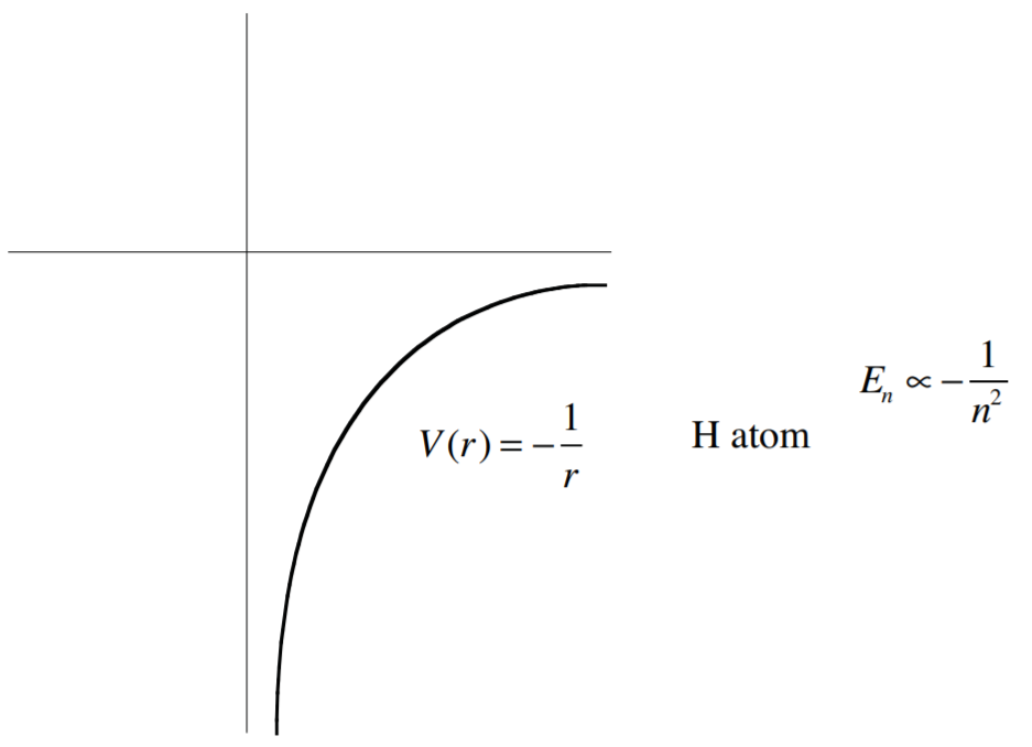
We have several kind of potential energy functions in atoms and molecules.
.png?revision=1&size=bestfit&width=306&height=222)
\(E_{n} = \propto n^{2}\)
particle in infinite-wall finite-length box (also particle on a ring)
Level pattern tells us quantitatively what kind of system we have.
Level splitting tell us quantitatively what are the properties of the class of system we have.
Rigid rotor
.png?revision=1)
\(E_{n} \propto n(n +1)\)
Harmonic Oscillator
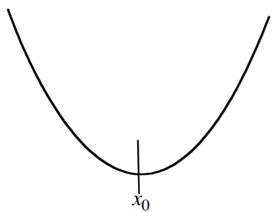.png?revision=1&size=bestfit&width=364&height=280)
\[V(x) = \frac{1}{2}kx^{2}\]
\[E_{n} = \propto (n+\frac{1}{2})\]
The pattern of the energy levels tells us which underlying microscopic structure we are dealing with.
Typical interatomic potential energy:
.png?revision=1&size=bestfit&width=596&height=265)
We will use \(x\) rather than \(R\) here.
Expand the potential energy function as a power series:
\[X - X_{0} \equiv x\]
\[V(x) = V(0) + \frac{dV}{dx}|_{x=0} + \dfrac{d^{2}V}{dx^{2}}|_{x=0}\frac{x^{2}}{2}+\frac{d^{3}V}{dx^{2}}\frac{x^{3}}{6}\]
For small x, OK to ignore terms of higher order than \(x^{2}\). [What do we know about \(\frac{dV}{dx}\) at the minimum of any V(x)?]
Example \(\PageIndex{1}\): Morse Potential
\(V(x) = D_{e}[1-e^{-ax}]^{2} = D_{e}[1-\overbrace{2e^{-ax}}^{\scriptsize[1-ax+\frac{a^{2}x^{2}}{2}+...]}+\overbrace{e^{-2ax}}^{\scriptsize[1-2ax+\frac{4a^{2}x^{2}}{2}+...]}]\)
Some Algebra
\( = V(0)+\underbrace{0}_{\text{Why physically} \\ \text{is there} \\ \text{no linear} \\ \text{in x term?} }+a^{2}D_{e}x^{2}-a^{3}D_{e}x^{3}+\frac{7}{12} a^{4} D_{e} x^{4}+... \)
\(V(\infty = D_{e})\)(dissociation energy),\(V(0) = 0\).
If \(ax\ll 1\), \(V(x)\approx V(0)+ ((D_{e})a^{2})x^{2}\). A very good starting point for the molecular vibrational potential energy curve.
Call \(D_{e}a^{2} = k/2\). Ignore the \(x^{3}\) and \(x^{4}\) terms.
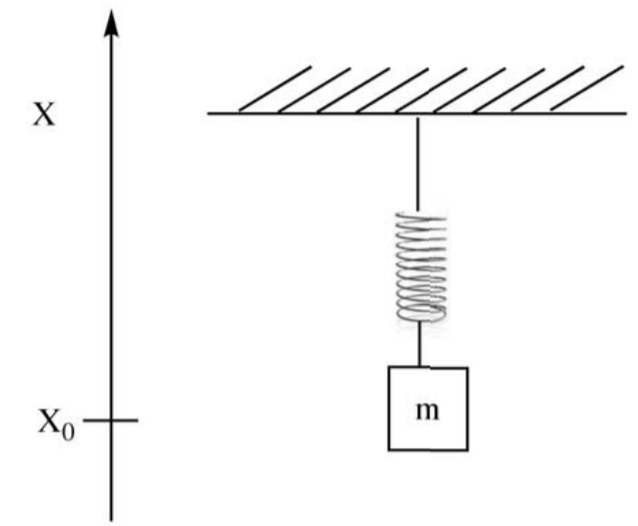
Hooke's Law
Let's first focus on a simple harmonic oscillator in the classical mechanics.
.png?revision=1&size=bestfit&width=300&height=248)
\[F = \underbrace {-k(X-X_{0})}_\text{force is - gradient of potential}\]
When \(X>X_{0}\),Force pushes mass back down toward \(X_{0}\)
\[F = -\frac{dV}{dX}\]
When \(X<X_{0}\), Force pulls mass back up towards \(X_{0}\)
\(\therefore V(x) = \frac{1}{2}k(X-X_{0})^2\)
Newton's Equation:
\[F = ma = m \frac{d^{2}(X-X_{0})}{dt^{2}} = -k(X-X_{0})\]
where \(x \equiv X-X_{0}\).
Substitute and rearrange
\(\frac{d^{2}x}{dt^{2}} = -\frac{k}{m}x\), \(2^{nd}\) order ordinary linear differential equation: solution contains two linearly independent terms, each multiplied by one of 2 constants to be determined
\[x(t) = A\sin \left(\frac{k}{m} \right)^{\frac{1}{2}} t + B\cos \left(\frac{k}{m} \right)^{\frac{1}{2}} t \]
It is customary to write
\[\left(\frac{k}{m} \right)^{\frac{1}{2}} = \omega.\]
(\(\omega\) is conventionally used to specify an angular frequency: radians/ second).
Why?
What is frequency of oscillation? \(\tau\) is the period of oscillation.
\[x(t+\tau)=x(t)= A\sin\left[\left(\frac{k}{m}\right)^{\frac{1}{2}} t \right] + B\cos\left[\left(\frac{k}{m} \right)^{\frac{1}{2}} t \right] = A\sin \left[\left(\frac{k}{m} \right)^{\frac{1}{2}} (t+\tau) \right] + B\cos \left[\left(\frac{k}{m} \right)^{\frac{1}{2}} (t+\tau) \right]\]
requires
\(\left(\frac{k}{m}\right)^{\frac{1}{2}}\tau = 2\pi\), \(v = \frac{1}{\tau}\) where \(\tau\) is period.
\(\tau = \frac{2\pi}{\omega}=\frac{2\pi}{2\pi v} = \frac{1}{v}\) as required.
How long does one full oscillation take?
We have sin, cos functions of \((\frac{k}{m})^{\frac{1}{2}}\) \(t = \omega t\)
when argument of sin or cos goes from 0 to \(2\pi\), we have one period of oscillation.
\[2\pi = \left(\frac{k}{m}\right)^{\frac{1}{2}}, \tau = \omega \tau\]
\[\tau = \frac{2\pi}{\omega}=\frac{1}{v}\]
So everything makes sense.
\(\omega\) is "angular frequency" (radians/sec).
\(v\) is ordinary frequency (cycles/sec).
\(\tau\) is period (sec).
\[x(t)=A\sin\omega t + B\cos\omega t\]
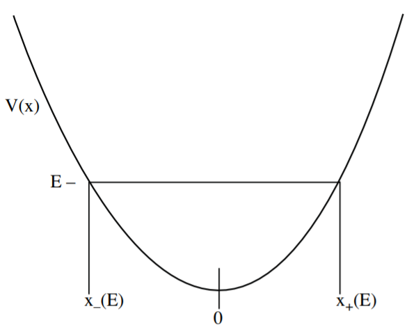
Need to get A, B from initial conditions:
.png?revision=1&size=bestfit&width=300&height=245)
[e.g. starting at a \(\overbrace{\text{turning point}}^{ASK!}\) where \(E=V(x_{\pm})=(1/2)kx_{\pm}^{2}\) and \( E \Rightarrow \pm(\frac{2E}{k})^{\frac{1}{2}} = x_{\pm}\)]
Initial amplitude of oscillation depends on the strength of the pluck!
If we start at \(x_{+}\) at t = 0, (the sine term is zero at t = 0, the cosine terms is B at t = 0)
\[x(0) = (\frac{2E}{k})^{\frac{1}{2}} \Rightarrow B = (\frac{2E}{k})^{\frac{1}{2}})\]
Note that the frequency of oscillation does not depend on initial amplitude. To get A for initial condition x(0)=\(x_{+}\), look at \(t=\tau /4\), where \(x(\tau /4)\) = 0. Find A = 0.
Alternatively, we can use frequency, phase form. For \(x(0) = x_{+}\) initial condition:
\[x(t) = C\sin \left( \left(\frac{k}{m} \right)^{\frac{1}{2}} t + \phi \right) \]
if \(x(0) = x_{+} = \left(\frac{2E}{k} \right)^{\frac{1}{2}}\)
C = \( \left(\frac{2E}{k} \right)^{\frac{1}{2}}\), \(\phi = -\pi /2\)
We are done. Now explore Quantum Mechanics - relevant stuff.
Quantum Mechanics
What is:
Oscillation Frequency
Kinetic Energy \(T(t)\), \(\overline{T}\)
Potential Energy \(V(t)\), \(\overline{V}\)
Period \(\tau\)?
Oscillation Frequency:
\[v = \frac{\omega}{2\pi}\] independent of E
Kinetic Energy:
\[T(t) = \frac{1}{2}mv(t)^{2}\]
\[x(t) = \left[\frac{2E}{k} \right]^{\frac{1}{2}}\sin \left[\omega t + \phi \right]\]
take derivative of x(t) with respect to t,
\[v(t) = \omega \left[\frac{2E}{k} \right]^{\frac{1}{2}}\cos \left[\omega t + \phi \right]\]
\[T(t) = \frac{1}{2}m\underbrace{\omega ^{2}}_{\scriptsize{k/m}} \left[\frac{2E}{k} \right]\cos^2 \left[\omega t + \phi \right]\]
\[E\cos^2 (\omega t + \phi)\]
Now some time averaged quantities:
\[\langle{T}\rangle = \overline{T} = E\frac{\int_0^\tau dt \cos^{2}(\omega t + \phi)}{\tau}\]
= E/2. Recall \(\tau = \frac{2 \pi}{\omega}\).
\[V(t) = \frac{1}{2} kx^{2} = \frac{k}{2} \left(\frac{2E}{k}\right) \sin^{2} (\omega t + \phi)\]
Calculate \(\langle{V}\rangle\) by \(\int_0^\tau dt\) or by simple algebra, below
\(= Esin^{2}(\omega t + \phi)\)
\(E = T(t)+V(t)= \overline{T}+ \overline{V}\)
\(\overline{V} = E/2\)
Really neat that \(\overline{T} = \overline{V} = E/2\).
Energy is being exchanged between \(T\) and \(V\). They oscillate \(\pi / 2\) out of phase:
\[V(t) = T\left(t - \frac{\tau}{4}\right)\]
V lags T.
What about x(t) and p(t) when x is near the turning point?
\[x(t) = \left[\frac{2E}{k} \right]^{\frac{1}{2}} \cos \omega t\]
where \(x(t=0) = x_{+}\).
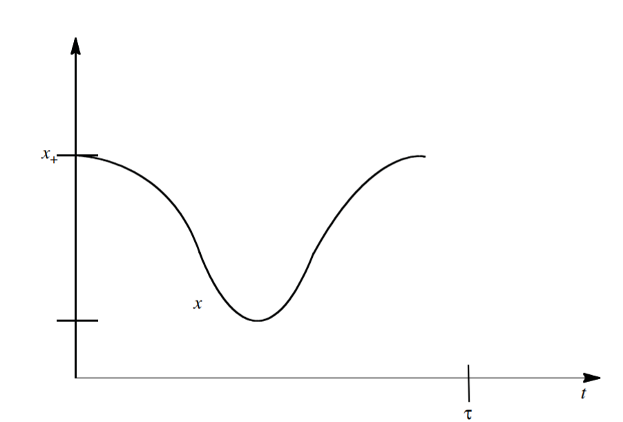.png?revision=1&size=bestfit&width=320&height=217)
\(x\) changing slowly near \(x\) turning point
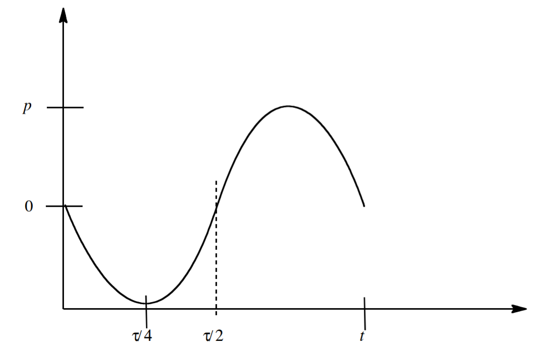.png?revision=1&size=bestfit&width=330&height=221)
\(p\) changing fastest near \(x\) turning point
Insights for wavepacket dynamics. We will see that "survival probability" \(|\Psi^{*}(x,t)\Psi(x,0)|^{2}\) decays near t.p. mostly \(\hat{p}\) rather than \(\hat{x}\).
What about time-averages of \(x,x^{2},p,p^{2}\)?
\( \left. \begin{array} \\ \langle{x}\rangle = 0 \\ \langle{p}\rangle = 0 \end{array} \right\} \text{is the HO potential moving in space?}\)
\[x^{2} = V(x)/ \frac{k}{2}\]
take t-average
\[\langle{x^{2}}\rangle=\frac{2}{k}\langle{v(x)}\rangle=\frac{2}{k}\frac{E}{2}=\frac{E}{k}\]
\[p^{2}=2mT\]
\[\langle{p^{2}}\rangle=2m\frac{E}{2}= mE\]
\[\Delta x = \langle{x^{2}- \langle{x}\rangle ^{2}}\rangle ^ {\frac{1}{2}}=(E/k)^{\frac{1}{2}}\]
\[\Delta p = \langle{p^{2}-\langle{p}\rangle^{2}}\rangle^{\frac{1}{2}}=(mE)^{\frac{1}{2}}\]
\[\Delta x \Delta p = E \left(\frac{m}{k}\right)^{\frac{1}{2}} = E/ \omega \text{ Small at low E}\].
We will see an uncertainty relationship between x and p in Quantum Mechanics.
Probability of finding oscillation between x and x + dx: consider one and half period, oscillator going from left to right turning point.
\[P(x)dx = \frac{time(x,x+dx)}{\tau / 2} = \frac{\frac{distance}{velocity}}{\frac{1}{2}\frac{2 \pi}{\omega}}\]
\(= \frac{\frac{dx}{v(x)}}{\frac{2 \pi}{2 \omega}}=\frac{2 \omega}{v(x)2 \pi}dx\)
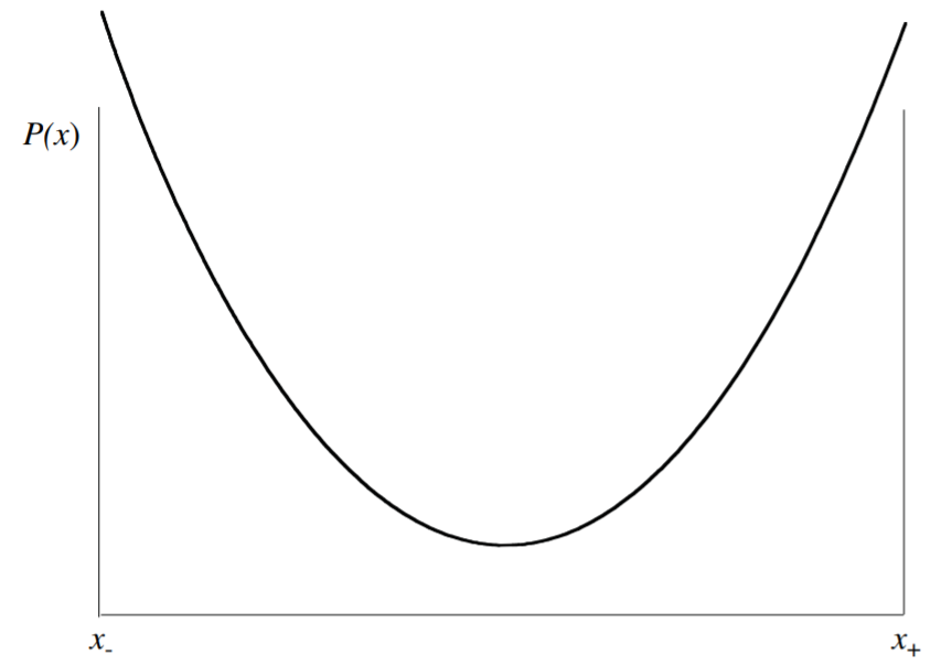.png?revision=1&size=bestfit&width=235&height=167)
large probability at turning point. Goes to \(\infty\) at \(x_{\pm}\).
Minimum probability at x = 0.
In Quantum Mechanics, we will see that \(P(x_{\pm})\) does not blow u and there is some probability outside the classically allowed region. Tunneling.
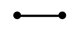
NON Lecture: Spring with Mass (Non Lecture)
Next we want to go from one mass on an anchored spring to two masses connected by a spring
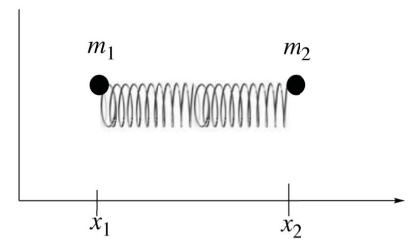.png?revision=1&size=bestfit&width=325&height=196)
F = ma for each mass
\[m_{1} \frac{d^{2}x_{1}}{dt^{2}} = k(x_{2}-x_{1} - {\it{l}_{0}} )\]
Where \(\it{l}_{0}\) is the length of the spring at rest, i.e. when \(x_{2} - x_{1} = \it{l}_{0}\)
\[m_{2} \frac{d^{2}x_{2}}{dt^{2}} = -k(x_{2}-x_{1} - {\it{l}_{0}} )\]
2 coupled differential equations.
Uncouple them easily, as follows:
Add the 2 equations:
\(m_{1} \frac{d^{2}x_{1}}{dt^{2}} + m_{2} \frac{d^{2}x_{2}}{dt^{2}}=\frac{d^{2}}{dt^{2}} \underbrace{(m_{1}x_{1}+m_{2}x_{2})}_{\text{we will see that}\\ \text{this is at worst}\\ \text{proportional}\\ \text{to t}}=0\)
Define a center of mass coordinate.
\[\frac{m_{1}x_{1} + m_{2}x_{2}}{M} = X\]
\[M = m_{1} + m_{2}\]
replace \(m_{1}x_{1} + m_{2}x_{2}\) by MX
\(M\frac{d^{2}X}{dt^{2}}=0\)
integrate once with respect to t
\(\frac{dX}{dt}(t) = \text{const}\).
The center of mass is moving at constant velocity — no force acting.
Next find a new differential equation expressed in terms of the relative coordinate.
\[x = x_{2} - x_{1} - \it{l}_{0}\]
Divide the first differential equation by \(m_{1}\), the second by \(m_{2}\), and subtract the first from the second:
\(\frac{d^{2}x_{2}}{dt^{2}}-\frac{d^{2}x_{1}}{dt^{2}} = -\frac{k}{m_{2}}(x_{2} - x_{1} - {\it{l}_{0}} )-\frac{k}{m_{1}}(x_{2} - x_{1} - {\it {l}_{0}} )\)
\(\frac{d^{2}}{dt^2}(x_{2}-x_{1})=-k\left(\frac{1}{m_{2}}+\frac{1}{m_{1}}\right)(x_{2} - x_{1} - {\it{l}_{0}} )\)
\(= -k \left(\frac{m_{1}+m_{2}}{m_{1}m_{2}}\right)(x_{2} - x_{1} - {\it{l}_{0}} )\)
\[\mu =\frac{m_{1}m_{2}}{m_{1}+m_{2}}\]
\(\frac{d^{2}}{dt^2}\underbrace{(x_{2}-x_{1})}_{\text{killed by}\\ \text{derivative}\\=x+{\it{l}_0}}=-\frac{k}{\mu}\underbrace{(x_{2} - x_{1} - \it{l}_{0}) = -\frac{k}{\mu}x}_{\text{x is displacement} \\ \text{from equilibrium}}\)
We get a familiar looking equation fro the intermolecular displacement from equilibrium.
\[\mu\frac{d^{2}x}{dt^{2}}+kx = 0\]
Everything is the same as the one-mass-on-a-spring problem except m → μ.
Next time: Quantum Mechanical Harmonic Oscillator
\[H = \frac{\hat{p}^{2}}{2 \mu}+\frac{1}{2}k \hat{x}^{2}\]
note that this differential operator does not have time in it!
We will see particle-like motion for harmonic oscillator when we consider the Time Dependent Schrödinger equation (Lecture #10) and Ψ(x,t) is a particle-like state.
\(\Psi(x,t)\) where \(\Psi(x,0) = \sum \limits_{v=0}^{\infty} C_{v}\Psi_{v}\)
in the \(4^{th}\) lecture on Harmonic Oscillators (Lecture #11).