Headspace analysis
- Page ID
- 61201
\( \newcommand{\vecs}[1]{\overset { \scriptstyle \rightharpoonup} {\mathbf{#1}} } \)
\( \newcommand{\vecd}[1]{\overset{-\!-\!\rightharpoonup}{\vphantom{a}\smash {#1}}} \)
\( \newcommand{\dsum}{\displaystyle\sum\limits} \)
\( \newcommand{\dint}{\displaystyle\int\limits} \)
\( \newcommand{\dlim}{\displaystyle\lim\limits} \)
\( \newcommand{\id}{\mathrm{id}}\) \( \newcommand{\Span}{\mathrm{span}}\)
( \newcommand{\kernel}{\mathrm{null}\,}\) \( \newcommand{\range}{\mathrm{range}\,}\)
\( \newcommand{\RealPart}{\mathrm{Re}}\) \( \newcommand{\ImaginaryPart}{\mathrm{Im}}\)
\( \newcommand{\Argument}{\mathrm{Arg}}\) \( \newcommand{\norm}[1]{\| #1 \|}\)
\( \newcommand{\inner}[2]{\langle #1, #2 \rangle}\)
\( \newcommand{\Span}{\mathrm{span}}\)
\( \newcommand{\id}{\mathrm{id}}\)
\( \newcommand{\Span}{\mathrm{span}}\)
\( \newcommand{\kernel}{\mathrm{null}\,}\)
\( \newcommand{\range}{\mathrm{range}\,}\)
\( \newcommand{\RealPart}{\mathrm{Re}}\)
\( \newcommand{\ImaginaryPart}{\mathrm{Im}}\)
\( \newcommand{\Argument}{\mathrm{Arg}}\)
\( \newcommand{\norm}[1]{\| #1 \|}\)
\( \newcommand{\inner}[2]{\langle #1, #2 \rangle}\)
\( \newcommand{\Span}{\mathrm{span}}\) \( \newcommand{\AA}{\unicode[.8,0]{x212B}}\)
\( \newcommand{\vectorA}[1]{\vec{#1}} % arrow\)
\( \newcommand{\vectorAt}[1]{\vec{\text{#1}}} % arrow\)
\( \newcommand{\vectorB}[1]{\overset { \scriptstyle \rightharpoonup} {\mathbf{#1}} } \)
\( \newcommand{\vectorC}[1]{\textbf{#1}} \)
\( \newcommand{\vectorD}[1]{\overrightarrow{#1}} \)
\( \newcommand{\vectorDt}[1]{\overrightarrow{\text{#1}}} \)
\( \newcommand{\vectE}[1]{\overset{-\!-\!\rightharpoonup}{\vphantom{a}\smash{\mathbf {#1}}}} \)
\( \newcommand{\vecs}[1]{\overset { \scriptstyle \rightharpoonup} {\mathbf{#1}} } \)
\(\newcommand{\longvect}{\overrightarrow}\)
\( \newcommand{\vecd}[1]{\overset{-\!-\!\rightharpoonup}{\vphantom{a}\smash {#1}}} \)
\(\newcommand{\avec}{\mathbf a}\) \(\newcommand{\bvec}{\mathbf b}\) \(\newcommand{\cvec}{\mathbf c}\) \(\newcommand{\dvec}{\mathbf d}\) \(\newcommand{\dtil}{\widetilde{\mathbf d}}\) \(\newcommand{\evec}{\mathbf e}\) \(\newcommand{\fvec}{\mathbf f}\) \(\newcommand{\nvec}{\mathbf n}\) \(\newcommand{\pvec}{\mathbf p}\) \(\newcommand{\qvec}{\mathbf q}\) \(\newcommand{\svec}{\mathbf s}\) \(\newcommand{\tvec}{\mathbf t}\) \(\newcommand{\uvec}{\mathbf u}\) \(\newcommand{\vvec}{\mathbf v}\) \(\newcommand{\wvec}{\mathbf w}\) \(\newcommand{\xvec}{\mathbf x}\) \(\newcommand{\yvec}{\mathbf y}\) \(\newcommand{\zvec}{\mathbf z}\) \(\newcommand{\rvec}{\mathbf r}\) \(\newcommand{\mvec}{\mathbf m}\) \(\newcommand{\zerovec}{\mathbf 0}\) \(\newcommand{\onevec}{\mathbf 1}\) \(\newcommand{\real}{\mathbb R}\) \(\newcommand{\twovec}[2]{\left[\begin{array}{r}#1 \\ #2 \end{array}\right]}\) \(\newcommand{\ctwovec}[2]{\left[\begin{array}{c}#1 \\ #2 \end{array}\right]}\) \(\newcommand{\threevec}[3]{\left[\begin{array}{r}#1 \\ #2 \\ #3 \end{array}\right]}\) \(\newcommand{\cthreevec}[3]{\left[\begin{array}{c}#1 \\ #2 \\ #3 \end{array}\right]}\) \(\newcommand{\fourvec}[4]{\left[\begin{array}{r}#1 \\ #2 \\ #3 \\ #4 \end{array}\right]}\) \(\newcommand{\cfourvec}[4]{\left[\begin{array}{c}#1 \\ #2 \\ #3 \\ #4 \end{array}\right]}\) \(\newcommand{\fivevec}[5]{\left[\begin{array}{r}#1 \\ #2 \\ #3 \\ #4 \\ #5 \\ \end{array}\right]}\) \(\newcommand{\cfivevec}[5]{\left[\begin{array}{c}#1 \\ #2 \\ #3 \\ #4 \\ #5 \\ \end{array}\right]}\) \(\newcommand{\mattwo}[4]{\left[\begin{array}{rr}#1 \amp #2 \\ #3 \amp #4 \\ \end{array}\right]}\) \(\newcommand{\laspan}[1]{\text{Span}\{#1\}}\) \(\newcommand{\bcal}{\cal B}\) \(\newcommand{\ccal}{\cal C}\) \(\newcommand{\scal}{\cal S}\) \(\newcommand{\wcal}{\cal W}\) \(\newcommand{\ecal}{\cal E}\) \(\newcommand{\coords}[2]{\left\{#1\right\}_{#2}}\) \(\newcommand{\gray}[1]{\color{gray}{#1}}\) \(\newcommand{\lgray}[1]{\color{lightgray}{#1}}\) \(\newcommand{\rank}{\operatorname{rank}}\) \(\newcommand{\row}{\text{Row}}\) \(\newcommand{\col}{\text{Col}}\) \(\renewcommand{\row}{\text{Row}}\) \(\newcommand{\nul}{\text{Nul}}\) \(\newcommand{\var}{\text{Var}}\) \(\newcommand{\corr}{\text{corr}}\) \(\newcommand{\len}[1]{\left|#1\right|}\) \(\newcommand{\bbar}{\overline{\bvec}}\) \(\newcommand{\bhat}{\widehat{\bvec}}\) \(\newcommand{\bperp}{\bvec^\perp}\) \(\newcommand{\xhat}{\widehat{\xvec}}\) \(\newcommand{\vhat}{\widehat{\vvec}}\) \(\newcommand{\uhat}{\widehat{\uvec}}\) \(\newcommand{\what}{\widehat{\wvec}}\) \(\newcommand{\Sighat}{\widehat{\Sigma}}\) \(\newcommand{\lt}{<}\) \(\newcommand{\gt}{>}\) \(\newcommand{\amp}{&}\) \(\definecolor{fillinmathshade}{gray}{0.9}\)Headspace analysis can be loosely defined as the analysis of characteristic volatile compounds associated with liquids or solids without direct sampling of the matrix. It is regarded therefore as a secondary method from which the original component concentrations can be determined by calibration. Typical samples can include water, effluents, soil, food, and beverages. The purpose of the analysis can be to evaluate and identify individual components or to relate chromatographic profiles to odour or aroma characteristics. Most manufacturers provide automatic equipment for many of these applications, and include air analyzers, water analyzers, automatic headspace analyzers, thermal desorbers, and purge and trap analyzers.
Basic headspace sampling techniques
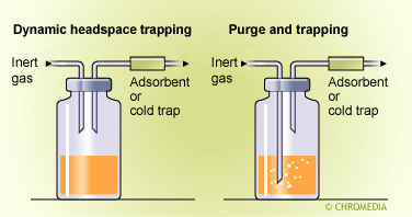
The sample itself is often in an unsuitable state for direct GC and so without headspace sampling it would require considerable sample pretreatment and cleanup before it could be applied to a GC column. The volatiles comprising the headspace are therefore sampled and chromatographed, and calibration procedures are employed to convert the measured component concentrations into values associated with the original sample. Several techniques are used for headspace sampling and for the subsequent handling before the analysis.
Types of headspace sampling
There are three essential types of sampling procedure for headspace analysis, viz, static headspace, dynamic headspace, and purge methods. These are illustrated by the diagrams and include illustrations of the methods of sample recovery, solvent extraction, thermal desorption, and cold trapping.
Headspace equilibrium
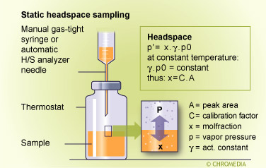
Static headspace sampling is the simplest method, particularly when carried out manually with a gas-tight syringe. For this purpose the sample must be thermostatted and allowed to reach an equilibrium situation. The headspace sample should be small in comparison with the total headspace volume to avoid the action of sampling from changing the sample characteristics, and the sampled volume must be compatible with the capillary column and its operating conditions. Gas samples of 10-2000 µl are possible in this way provided a split is used and the column is preferably operated under programmed conditions. Alternatively a splitless method can be used in conjunction with a liquid nitrogen cold trap at the start of the column, similar to the purge and trap equipment shown in its schematic diagram. Because of the relatively small volumes obtained in static sampling, this method is unlikely to be successful for determining concentrations in the ppm-ppb range or lower.
Automatic headspace

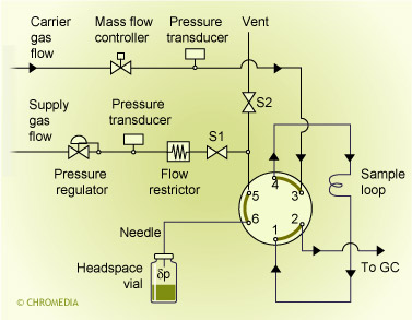
Commercial automatic headspace samplers are manufactured by many of the commercial suppliers and these are largely based on the static headspace principle. Samples are usually contained in thermostatted vials in a carousel for multiple analyses, and headspace samples are taken automatically by penetration of a septum by a needle.
The concentration of each component in the headspace is related its concentration in the liquid or solid sample according to Henry's law by:
\[C0_{(liquid)} = [ Ci_{(gas)} \times (KVL + VG)] / VL\]
Where C0(liquid)= original concentration of component in liquid, C(gas)=concentration in the headspace gas; K=partition coefficient; VL= volume of liquid; and VG= volume of headspace gas.
This relationship will only hold provided Henry's law is applicable and for accuracy a careful calibration should be carried out over the range of relevant concentrations. A further complication could arise if some of the required compounds associate with the sample matrix to give higher partition coefficients than otherwise.
Automatic headspace (continued)
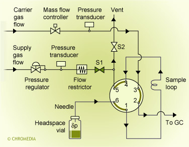
In an automated system the sample vial is heated during a fixed period of time. After that the sample vial is pressurized. By switching the valve the headspace vapour flows to the sample loop and injection takes place by switching the 6-port valve again. Injection can be direct (wide-bore columns only) or split. Pressures, times, temperatures must be controlled carefully to obtain reproducible results.
Besides pressure and temperature, also the composition of the sample matrix has a big effect on the equilibrium between the sample and the headspace. Matrix effects are depending on homogeneity, salt concentration, solvent type, solid particles, adsorption effects and pH values of aqueous matrices. These factors are important for the choice of the right range of standards for calibration, one of the major problems in quantitative headspace analysis. Not always a good blank sample is available. Spiking of (solid) samples is an option, but not very reliable and reproducible.
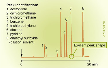
A well known application of headspace analysis is the determination of residual solvents in pharmaceutical products. Also the analysis of alcohol in blood can be done with headspace down to ppm levels. In principle the (dirty) matrix of the sample is not injected, so both the injector and the column will remain clean even after numerous injections. Also the chromatogram does contain only a small solvent peak, which results in clean chromatograms.
Headspace analysis of solvent residues
