
9.1: Overview of Titrimetry
- Page ID
- 5617

\( \newcommand{\vecs}[1]{\overset { \scriptstyle \rightharpoonup} {\mathbf{#1}} } \)
\( \newcommand{\vecd}[1]{\overset{-\!-\!\rightharpoonup}{\vphantom{a}\smash {#1}}} \)
\( \newcommand{\id}{\mathrm{id}}\) \( \newcommand{\Span}{\mathrm{span}}\)
( \newcommand{\kernel}{\mathrm{null}\,}\) \( \newcommand{\range}{\mathrm{range}\,}\)
\( \newcommand{\RealPart}{\mathrm{Re}}\) \( \newcommand{\ImaginaryPart}{\mathrm{Im}}\)
\( \newcommand{\Argument}{\mathrm{Arg}}\) \( \newcommand{\norm}[1]{\| #1 \|}\)
\( \newcommand{\inner}[2]{\langle #1, #2 \rangle}\)
\( \newcommand{\Span}{\mathrm{span}}\)
\( \newcommand{\id}{\mathrm{id}}\)
\( \newcommand{\Span}{\mathrm{span}}\)
\( \newcommand{\kernel}{\mathrm{null}\,}\)
\( \newcommand{\range}{\mathrm{range}\,}\)
\( \newcommand{\RealPart}{\mathrm{Re}}\)
\( \newcommand{\ImaginaryPart}{\mathrm{Im}}\)
\( \newcommand{\Argument}{\mathrm{Arg}}\)
\( \newcommand{\norm}[1]{\| #1 \|}\)
\( \newcommand{\inner}[2]{\langle #1, #2 \rangle}\)
\( \newcommand{\Span}{\mathrm{span}}\) \( \newcommand{\AA}{\unicode[.8,0]{x212B}}\)
\( \newcommand{\vectorA}[1]{\vec{#1}} % arrow\)
\( \newcommand{\vectorAt}[1]{\vec{\text{#1}}} % arrow\)
\( \newcommand{\vectorB}[1]{\overset { \scriptstyle \rightharpoonup} {\mathbf{#1}} } \)
\( \newcommand{\vectorC}[1]{\textbf{#1}} \)
\( \newcommand{\vectorD}[1]{\overrightarrow{#1}} \)
\( \newcommand{\vectorDt}[1]{\overrightarrow{\text{#1}}} \)
\( \newcommand{\vectE}[1]{\overset{-\!-\!\rightharpoonup}{\vphantom{a}\smash{\mathbf {#1}}}} \)
\( \newcommand{\vecs}[1]{\overset { \scriptstyle \rightharpoonup} {\mathbf{#1}} } \)
\( \newcommand{\vecd}[1]{\overset{-\!-\!\rightharpoonup}{\vphantom{a}\smash {#1}}} \)
\(\newcommand{\avec}{\mathbf a}\) \(\newcommand{\bvec}{\mathbf b}\) \(\newcommand{\cvec}{\mathbf c}\) \(\newcommand{\dvec}{\mathbf d}\) \(\newcommand{\dtil}{\widetilde{\mathbf d}}\) \(\newcommand{\evec}{\mathbf e}\) \(\newcommand{\fvec}{\mathbf f}\) \(\newcommand{\nvec}{\mathbf n}\) \(\newcommand{\pvec}{\mathbf p}\) \(\newcommand{\qvec}{\mathbf q}\) \(\newcommand{\svec}{\mathbf s}\) \(\newcommand{\tvec}{\mathbf t}\) \(\newcommand{\uvec}{\mathbf u}\) \(\newcommand{\vvec}{\mathbf v}\) \(\newcommand{\wvec}{\mathbf w}\) \(\newcommand{\xvec}{\mathbf x}\) \(\newcommand{\yvec}{\mathbf y}\) \(\newcommand{\zvec}{\mathbf z}\) \(\newcommand{\rvec}{\mathbf r}\) \(\newcommand{\mvec}{\mathbf m}\) \(\newcommand{\zerovec}{\mathbf 0}\) \(\newcommand{\onevec}{\mathbf 1}\) \(\newcommand{\real}{\mathbb R}\) \(\newcommand{\twovec}[2]{\left[\begin{array}{r}#1 \\ #2 \end{array}\right]}\) \(\newcommand{\ctwovec}[2]{\left[\begin{array}{c}#1 \\ #2 \end{array}\right]}\) \(\newcommand{\threevec}[3]{\left[\begin{array}{r}#1 \\ #2 \\ #3 \end{array}\right]}\) \(\newcommand{\cthreevec}[3]{\left[\begin{array}{c}#1 \\ #2 \\ #3 \end{array}\right]}\) \(\newcommand{\fourvec}[4]{\left[\begin{array}{r}#1 \\ #2 \\ #3 \\ #4 \end{array}\right]}\) \(\newcommand{\cfourvec}[4]{\left[\begin{array}{c}#1 \\ #2 \\ #3 \\ #4 \end{array}\right]}\) \(\newcommand{\fivevec}[5]{\left[\begin{array}{r}#1 \\ #2 \\ #3 \\ #4 \\ #5 \\ \end{array}\right]}\) \(\newcommand{\cfivevec}[5]{\left[\begin{array}{c}#1 \\ #2 \\ #3 \\ #4 \\ #5 \\ \end{array}\right]}\) \(\newcommand{\mattwo}[4]{\left[\begin{array}{rr}#1 \amp #2 \\ #3 \amp #4 \\ \end{array}\right]}\) \(\newcommand{\laspan}[1]{\text{Span}\{#1\}}\) \(\newcommand{\bcal}{\cal B}\) \(\newcommand{\ccal}{\cal C}\) \(\newcommand{\scal}{\cal S}\) \(\newcommand{\wcal}{\cal W}\) \(\newcommand{\ecal}{\cal E}\) \(\newcommand{\coords}[2]{\left\{#1\right\}_{#2}}\) \(\newcommand{\gray}[1]{\color{gray}{#1}}\) \(\newcommand{\lgray}[1]{\color{lightgray}{#1}}\) \(\newcommand{\rank}{\operatorname{rank}}\) \(\newcommand{\row}{\text{Row}}\) \(\newcommand{\col}{\text{Col}}\) \(\renewcommand{\row}{\text{Row}}\) \(\newcommand{\nul}{\text{Nul}}\) \(\newcommand{\var}{\text{Var}}\) \(\newcommand{\corr}{\text{corr}}\) \(\newcommand{\len}[1]{\left|#1\right|}\) \(\newcommand{\bbar}{\overline{\bvec}}\) \(\newcommand{\bhat}{\widehat{\bvec}}\) \(\newcommand{\bperp}{\bvec^\perp}\) \(\newcommand{\xhat}{\widehat{\xvec}}\) \(\newcommand{\vhat}{\widehat{\vvec}}\) \(\newcommand{\uhat}{\widehat{\uvec}}\) \(\newcommand{\what}{\widehat{\wvec}}\) \(\newcommand{\Sighat}{\widehat{\Sigma}}\) \(\newcommand{\lt}{<}\) \(\newcommand{\gt}{>}\) \(\newcommand{\amp}{&}\) \(\definecolor{fillinmathshade}{gray}{0.9}\)In titrimetry we add a reagent, called the titrant, to a solution containing another reagent, called the titrand, and allow them to react. The type of reaction provides us with a simple way to divide titrimetry into the following four categories: acid–base titrations, in which an acidic or basic titrant reacts with a titrand that is a base or an acid; complexometric titrations based on metal–ligand complexation; redox titrations, in which the titrant is an oxidizing or reducing agent; and precipitation titrations, in which the titrand and titrant form a precipitate.
Note
We are deliberately avoiding the term analyte at this point in our introduction to titrimetry. Although in most titrations the analyte is the titrand, there are circumstances where the analyte is the titrant. When discussing specific methods, we will use the term analyte where appropriate.
Despite the difference in chemistry, all titrations share several common features. Before we consider individual titrimetric methods in greater detail, let’s take a moment to consider some of these similarities. As you work through this chapter, this overview will help you focus on similarities between different titrimetric methods. You will find it easier to understand a new analytical method when you can see its relationship to other similar methods.
9.1.1 Equivalence Points and End points
If a titration is to be accurate we must combine stoichiometrically equivalent amount of titrant and titrand. We call this stoichiometric mixture the equivalence point. Unlike precipitation gravimetry, where we add the precipitant in excess, an accurate titration requires that we know the exact volume of titrant at the equivalence point, Veq. The product of the titrant’s equivalence point volume and its molarity, MT, is equal to the moles of titrant reacting with the titrand.
\[\textrm{moles of titrant}=M_\textrm T\times V_{\textrm{eq}}\]
If we know the stoichiometry of the titration reaction, then we can calculate the moles of titrand.
Unfortunately, for most titrations there is no obvious sign when we reach the equivalence point. Instead, we stop adding titrant when at an end point of our choosing. Often this end point is a change in the color of a substance, called an indicator, that we add to the titrand’s solution. The difference between the end point volume and the equivalence point volume is a determinate titration error. If the end point and the equivalence point volumes coincide closely, then the titration error is insignificant and it is safely ignored. Clearly, selecting an appropriate end point is critically important.
9.1.2 Volume as a Signal
Note
Instead of measuring the titrant’s volume, we may choose to measure its mass. Although we generally can measure mass more precisely than we can measure volume, the simplicity of a volumetric titration makes it the more popular choice.
Almost any chemical reaction can serve as a titrimetric method provided it meets the following four conditions. The first condition is that we must know the stoichiometry between the titrant and the titrand. If this is not the case, then we cannot convert the moles of titrant consumed in reaching the end point to the moles of titrand in our sample. Second, the titration reaction must effectively proceed to completion; that is, the stoichiometric mixing of the titrant and the titrand must result in their reaction. Third, the titration reaction must occur rapidly. If we add the titrant faster than it can react with the titrand, then the end point and the equivalence point will differ significantly. Finally, there must be a suitable method for accurately determining the end point. These are significant limitations and, for this reason, there are several common titration strategies.
Note
Depending on how we are detecting the endpoint, we may stop the titration too early or too late. If the end point is a function of the titrant’s concentration, then adding the titrant too quickly leads to an early end point. On the other hand, if the end point is a function of the titrant’s concentration, then the end point exceeds the equivalence point.
A simple example of a titration is an analysis for Ag+ using thiocyanate, SCN–, as a titrant.
\[\mathrm{Ag^+}(aq)+\mathrm{SCN^-}(aq)\rightleftharpoons\mathrm{Ag(SCN)}(s)\]
Note
This is an example of a precipitation titration. You will find more information about precipitation titrations in Section 9.5.
This reaction occurs quickly and with a known stoichiometry, satisfying two of our requirements. To indicate the titration’s end point, we add a small amount of Fe3+ to the analyte’s solution before beginning the titration. When the reaction between Ag+ and SCN– is complete, formation of the red-colored Fe(SCN)2+ complex signals the end point. This is an example of a direct titration since the titrant reacts directly with the analyte.
If the titration’s reaction is too slow, if a suitable indicator is not available, or if there is no useful direct titration reaction, then an indirect analysis may be possible. Suppose you wish to determine the concentration of formaldehyde, H2CO, in an aqueous solution. The oxidation of H2CO by I3–
\[\mathrm{H_2CO}(aq)+\ce{I_3^-}(aq)+\mathrm{3OH^-}(aq)\rightleftharpoons \mathrm{HCO_2^-}(aq) + \mathrm{3I^-}(aq) + \mathrm{2H_2O}(l)\]
is a useful reaction, but it is too slow for a titration. If we add a known excess of I3– and allow its reaction with H2CO to go to completion, we can titrate the unreacted I3– with thiosulfate, S2O32–.
\[\ce{I_3^-}(aq)+\mathrm{2S_2O_3^{2-}}(aq)\rightleftharpoons \mathrm{S_4O_6^{2-}}(aq) + \mathrm{3I^-}(aq)\]
Note
This is an example of a redox titration. You will find more information about redox titrations in Section 9.4.
The difference between the initial amount of I3– and the amount in excess gives us the amount of I3– reacting with the formaldehyde. This is an example of a back titration.
Calcium ion plays an important role in many environmental systems. A direct analysis for Ca2+ might take advantage of its reaction with the ligand ethylenediaminetetraacetic acid (EDTA), which we represent here as Y4–.
\[\mathrm{Ca^{2+}}(aq)+\mathrm Y^{4-}(aq)\rightleftharpoons \mathrm{CaY^{2-}}(aq)\]
Unfortunately, for most samples this titration does not have a useful indicator. Instead, we react the Ca2+ with an excess of MgY2–
\[\mathrm{Ca^{2+}}(aq) + \mathrm{MgY^{2-}}(aq)\rightleftharpoons \mathrm{CaY^{2-}}(aq) + \mathrm{Mg^{2+}}(aq)\]
releasing an amount of Mg2+ equivalent to the amount of Ca2+ in the sample.
Note
MgY2– is the Mg2+–EDTA metal–ligand complex. You can prepare a solution of MgY2– by combining equimolar solutions of Mg2+ and EDTA.
Because the titration of Mg2+ with EDTA
\[\mathrm{Mg^{2+}}(aq) + \mathrm{Y^{4-}}(aq)\rightleftharpoons \mathrm{MgY^{2-}}(aq)\]
has a suitable end point, we can complete the analysis.
Note
This is an example of a complexation titration. You will find more information about complexation titrations in Section 9.3.
The amount of EDTA used in the titration provides an indirect measure of the amount of Ca2+ in the original sample. Because the species we are titrating was displaced by the analyte, we call this a displacement titration.
If a suitable reaction involving the analyte does not exist it may be possible to generate a species that we can titrate. For example, we can determine the sulfur content of coal by using a combustion reaction to convert sulfur to sulfur dioxide
\[\mathrm S(s) + \mathrm O_2(g)\rightarrow \mathrm{SO_2}(g)\]
and then convert the SO2 to sulfuric acid, H2SO4, by bubbling it through an aqueous solution of hydrogen peroxide, H2O2.
\[\mathrm{SO_2}(g) + \mathrm{H_2O_2}(aq)\rightarrow \mathrm{H_2SO_4}(aq)\]
Titrating H2SO4 with NaOH
\[\mathrm{H_2SO_4}(aq) + \mathrm{2NaOH}(aq)\rightleftharpoons \mathrm{2H_2O}(l) + \mathrm{Na_2SO_4}(aq)\]
provides an indirect determination of sulfur.
Note
This is an example of an acid–base titration. You will find more information about acid–base titrations in Section 9.2.
9.1.3 Titration Curves
To find a titration’s end point, we need to monitor some property of the reaction that has a well-defined value at the equivalence point. For example, the equivalence point for a titration of HCl with NaOH occurs at a pH of 7.0. A simple method for finding the equivalence point is to continuously monitor the titration mixture’s pH using a pH electrode, stopping the titration when we reach a pH of 7.0. Alternatively, we can add an indicator to the titrand’s solution that changes color at a pH of 7.0.
Note
Why a pH of 7.0 is the equivalence point for this titration is a topic we will cover in Section 9.2.
Suppose the only available indicator changes color at an end point pH of 6.8. Is the difference between the end point and the equivalence point small enough that we can safely ignore the titration error? To answer this question we need to know how the pH changes during the titration.
A titration curve provides us with a visual picture of how a property of the titration reaction changes as we add the titrant to the titrand. The titration curve in Figure 9.1, for example, was obtained by suspending a pH electrode in a solution of 0.100 M HCl (the titrand) and monitoring the pH while adding 0.100 M NaOH (the titrant). A close examination of this titration curve should convince you that an end point pH of 6.8 produces a negligible titration error. Selecting a pH of 11.6 as the end point, however, produces an unacceptably large titration error.
Note
For the titration curve in Figure 9.1, the volume of titrant to reach a pH of 6.8 is 24.99995 mL, a titration error of –2.00×10⁻⁴%. Typically, we can only read the volume to the nearest ±0.01 mL, which means this uncertainty is too small to affect our results.
The volume of titrant to reach a pH of 11.6 is 27.07 mL, or a titration error of +8.28%. This is a significant error.
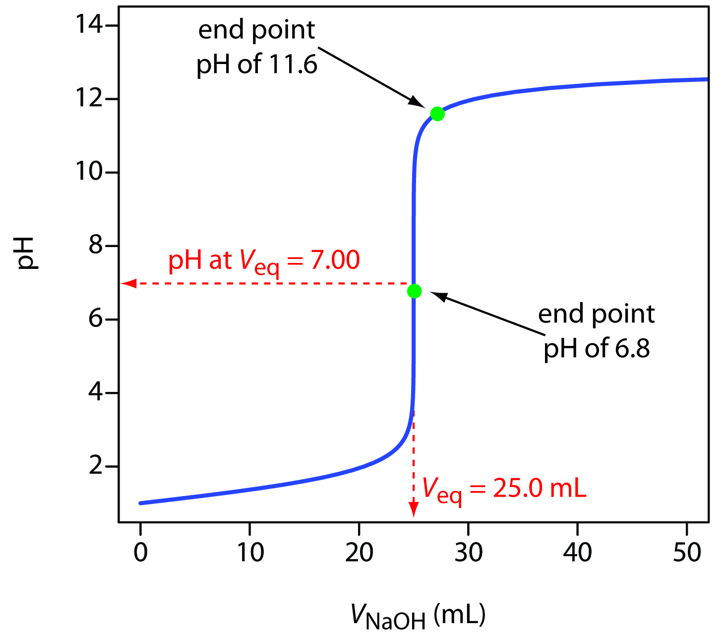
Figure 9.1 Typical acid–base titration curve showing how the titrand’s pH changes with the addition of titrant. The titrand is a 25.0 mL solution of 0.100 M HCl and the titrant is 0.100 M NaOH. The titration curve is the solid blue line, and the equivalence point volume (25.0 mL) and pH (7.00) are shown by the dashed red lines. The green dots show two end points. The end point at a pH of 6.8 has a small titration error, and the end point at a pH of 11.6 has a larger titration error.
The titration curve in Figure 9.1 is not unique to an acid–base titration. Any titration curve that follows the change in concentration of a species in the titration reaction (plotted logarithmically) as a function of the titrant’s volume has the same general sigmoidal shape. Several additional examples are shown in Figure 9.2.
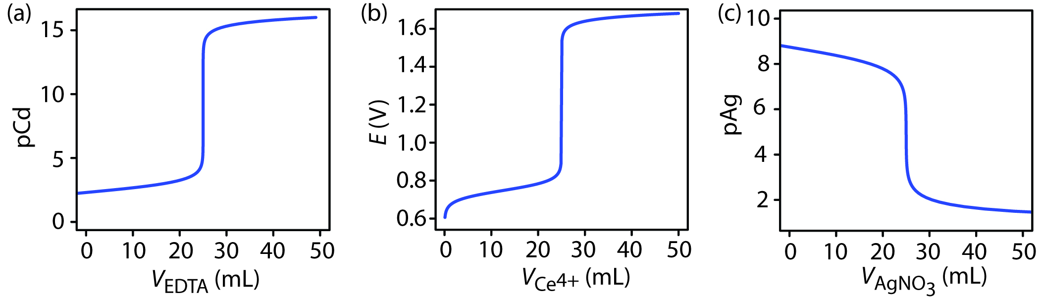
Figure 9.2 Additional examples of titration curves. (a) Complexation titration of 25.0 mL of 1.0 mM Cd2+ with 1.0 mM EDTA at a pH of 10. The y-axis displays the titrand’s equilibrium concentration as pCd. (b) Redox titration of 25.0 mL of 0.050 M Fe2+ with 0.050 M Ce4+ in 1 M HClO4. The y-axis displays the titration mixture’s electrochemical potential, E, which, through the Nernst equation is a logarithmic function of concentrations. (c) Precipitation titration of 25.0 mL of 0.10 M NaCl with 0.10 M AgNO3. The y-axis displays the titrant’s equilibrium concentration as pAg.
The titrand’s or the titrant’s concentration is not the only property we can use when recording a titration curve. Other parameters, such as the temperature or absorbance of the titrand’s solution, may provide a useful end point signal. Many acid–base titration reactions, for example, are exothermic. As the titrant and titrand react the temperature of the titrand’s solution steadily increases. Once we reach the equivalence point, further additions of titrant do not produce as exothermic a response. Figure 9.3 shows a typical thermometric titration curve with the intersection of the two linear segments indicating the equivalence point.
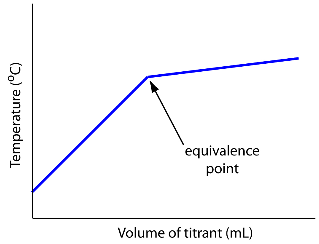
Figure 9.3 Example of a thermometric titration curve showing the location of the equivalence point.
9.1.4 The Buret
The only essential equipment for an acid–base titration is a means for delivering the titrant to the titrand’s solution. The most common method for delivering titrant is a buret (Figure 9.4). A buret is a long, narrow tube with graduated markings, equipped with a stopcock for dispensing the titrant. The buret’s small internal diameter provides a better defined meniscus, making it easier to read the titrant’s volume precisely. Burets are available in a variety of sizes and tolerances (Table 9.1), with the choice of buret determined by the needs of the analysis. You can improve a buret’s accuracy by calibrating it over several intermediate ranges of volumes using the method described in Chapter 5 for calibrating pipets. Calibrating a buret corrects for variations in the buret’s internal diameter.
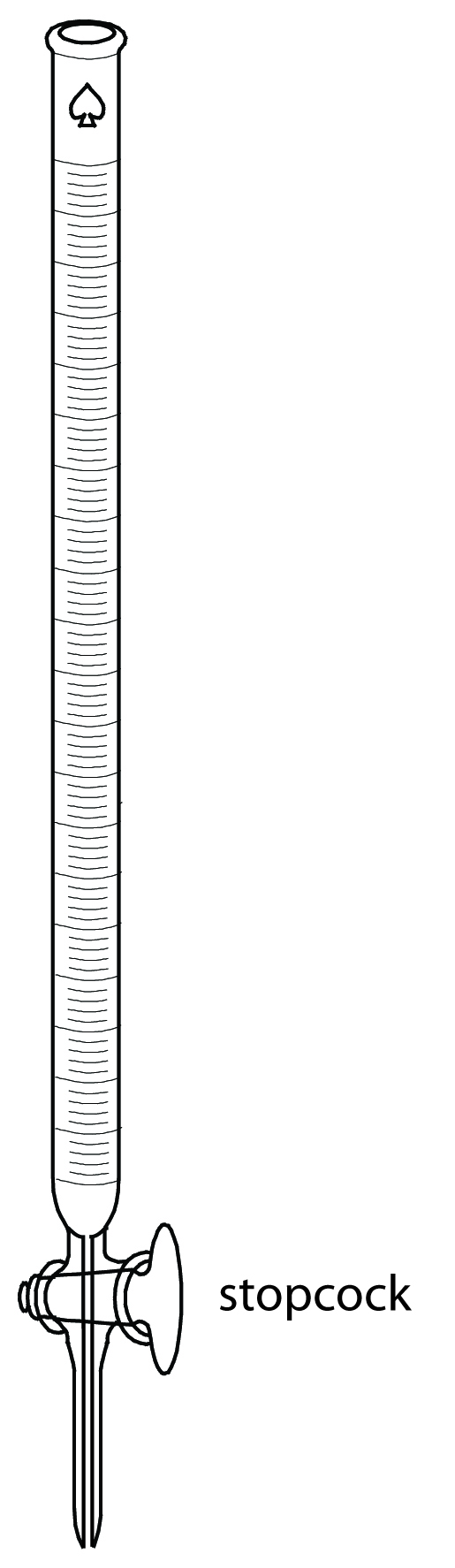
Figure 9.4 Typical volumetric buret. The stopcock is in the open position, allowing the titrant to flow into the titrand’s solution. Rotating the stopcock controls the titrant’s flow rate.
|
Volume (mL) |
Class |
Subdivision (mL) |
Tolerance (mL) |
|---|---|---|---|
|
5 |
A B |
0.01 0.01 |
±0.01 ±0.01 |
|
10 |
A B |
0.02 0.02 |
±0.02 ±0.04 |
|
25 |
A B |
0.1 0.1 |
±0.03 ±0.06 |
|
50 |
A B |
0.1 0.1 |
±0.05 ±0.10 |
|
100 |
A B |
0.2 0.2 |
±0.10 ±0.20 |
A titration can be automated by using a pump to deliver the titrant at a constant flow rate (Figure 9.5). Automated titrations offer the additional advantage of using a microcomputer for data storage and analysis.
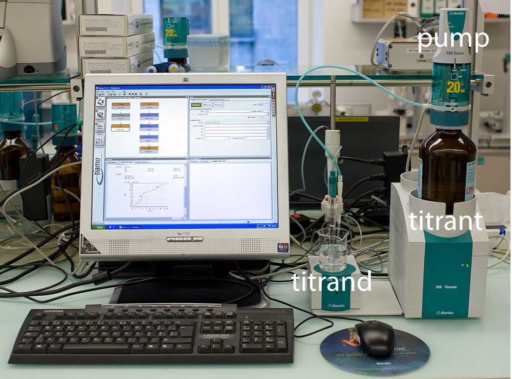
Figure 9.5 Typical instrumentation for an automated acid–base titration showing the titrant, the pump, and the titrand. The pH electrode in the titrand’s solution is used to monitor the titration’s progress. You can see the titration curve in the lower-left quadrant of the computer’s display. Modified from: Datamax (commons.wikipedia.org).