Part IV: Ways to Model Data

In Part III we made a distinction between a sample and a population, noting that a population is every member of a system that we could analyze and that a sample is the discrete subset of a population that we actually analyze. We collect and analyze samples with the hope that we can use their properties to deduce something about the population’s properties. We accomplish this by using suitable mathematical models.

Investigation 18.

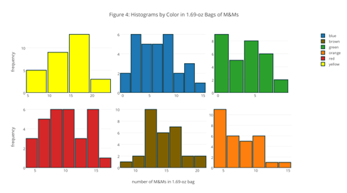
So, what does it mean to build a model? Consider the histograms in Figure 4. What property of the population are we attempting to model? What do your responses imply about the model’s general mathematical form? What does it mean to test a model and how might we accomplish this?

There are a variety of ways in which we might model our data, three of which we consider in this section: the binomial distribution, the Poisson distribution, and the normal distribution.

Binomial Distribution. A binomial distribution describes the probability, P, of a particular event, X, during a fixed number of trials, N, given the probability, p, that the event happens during a single trial. Mathematically, we express the binomial distribution as

\[P(X,N)=\dfrac{N!}{X!(N-X)!}\times p^X \times (1-p)^{N-X}\]

where ! is the factorial symbol. The theoretical mean, μ, and the theoretical variance, σ ², for a binomial distribution are

\[μ = Np \hspace{40px} σ^2 = Np (1 - p)\]

Investigation 19.

The box and whisker plot in Figure 1 includes data from the analysis of 30 samples of 1.69-oz bags of plain M&Ms. Collectively, the samples have 1699 M&Ms, of which 435 are yellow. If you pick one M&M at random from these 1699 M&Ms, what is the probability, p, that it is yellow? Suppose that this probability applies to the population of all plain M&Ms. If we draw a sample of five M&Ms from this population, what is the probability that the sample contains no yellow M&Ms? Repeat for each of 1–5 yellow M&Ms. Construct a histogram of your results and report the mean and the variance. Repeat this analysis for green M&Ms. Compare your two histograms and discuss their similarities and their differences. Using the data in Table 2, comment on the suitability of the binomial distribution for modeling the number of yellow M&Ms in samples of five M&Ms.

Poisson Distribution. The binomial distribution is useful if we wish to model the probability of finding a fixed number of yellow M&Ms in a sample of M&Ms of fixed size, but not the probability of finding a fixed number of yellow M&Ms in a single bag.

Investigation 20.

Explain why we cannot use the binomial distribution to model the distribution of yellow M&Ms in 1.69-oz bags of plain M&Ms.

To model the number of yellow M&Ms in packages of M&Ms, we use the Poisson distribution, which gives the probability of a particular event, X, given an average rate, λ, for that event. Mathematically, we express the Poisson distribution as

\[P(X,λ)=\dfrac{e^{-λ} λ^X}{X!}\]

The theoretical mean, μ, and the theoretical variance, σ ², are both equal to λ.

Investigation 21.

The histograms in Figure 4 include data from the analysis of 30 samples of 1.69-oz bags of plain M&Ms. Collectively, the samples have an average of 14.5 yellow M&Ms per bag. Suppose this rate applies to the population of all 1.69-oz bags of plain M&Ms. If you pick a 1.69-oz bag of plain M&Ms at random, what is the probability that it contains exactly 11 yellow M&Ms? Repeat for each of 0–29 yellow M&Ms. Construct a histogram that shows the actual distribution of bags of M&Ms for each of 0–29 yellow M&Ms, using a bin size of 1 unit, and overlay a line plot that shows the predicted distribution of bags; be sure to you use the same scale for each plot’s y-axis. Comment on your results.

Normal Distribution. The binomial distribution and the Poisson distribution are examples of discrete functions in that they predict the probability of a discrete event, such as finding exactly two green M&Ms in the next bag of M&Ms that we open. Not all data we might collect on M&Ms, however, is discrete.

Investigation 22.

Explain why we cannot use the binomial distribution or the Poisson distribution to model data for the net weight of M&Ms in Table 2.

To model the net weight of packages of M&Ms, we use the normal distribution, which gives the probability of obtaining a particular outcome from a population with a known mean, μ, and a known variance, σ ². Mathematically, we express the normal distribution as

\[P(X)=\dfrac{1}{\sqrt{2πσ^2}}e^{\large{-(X-μ)^2 ⁄2πσ^2}}\]

Figure 6 shows the normal distribution curves for μ = 0 and for variances of 25, 100, and 400.

Investigation 23.

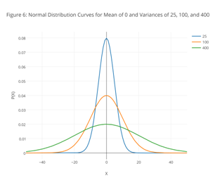
Using the curves in Figure 6 as an example, discuss the general features of a normal distribution, giving particular attention to the importance of variance. How do you think the areas under the three curves from -∞ to +∞ are related to each other? Why might this be important?

Because the equation for a normal distribution depends solely on the population’s mean, μ, and variance, σ ², the probability that a sample drawn from a population has a value between any two arbitrary limits is the same for all populations. For example, 68.26% of all samples drawn from a normally distributed population will have values within the range μ ± σ, and only 0.621% will have values greater than μ + 2.5σ; see Appendix 2 for further details.

Investigation 24.

Assuming that the mean, \(\bar{x}\), and the standard deviation, s, for the net weight of our samples of M&Ms are good estimates for the population’s mean, μ, and standard deviation, σ, what is the probability that the contents of a 1.69-oz bag of plain M&Ms selected at random will weigh less than the stated net weight of 1.69 oz? Suppose the manufacturer wants to reduce this probability to no more than 5%: How might they accomplish this?

For a binomial distribution, if N × p ≥ 5 and N × (1 - p) ≥ 5, then a normal distribution closely approximates a binomial distribution; the same is true for a Poisson distribution when λ ≥ 20.

Investigation 25.

Suppose we arrange to collect samples of plain M&Ms such that each sample contains 330 M&Ms—an amount roughly equivalent to a 10-oz bag of plain M&Ms—drawn from the same population as the data in Table 2. Can we model this data using a normal distribution in place of the binomial distribution or the Poisson distribution? What advantages are there in being able to use the normal distribution? How might you apply this to more practical analytical problems, such as determining the concentration of Pb²⁺ in soil?