5.3: Chemical shift in units of Hz and ppm

This Chapter introduces the other most common unit to measure and report the NMR resonance frequency: ppm, parts-per-million. We will consider examples when the frequency units of Hz (1/second) are the most justified choice and the opposite cases- when ppm’s should be used. We will also start describing quantitatively how raw NMR signal, S(t), depend on time t, initial current S₀, and two properties of the target nucleus: resonance frequency Ω (or ν) and relaxation rate R.

Learning Objectives

• Understand the dependence of frequency expressed in units of Hz from the instrumentation used (magnet strength)
• Define the magnet strength- independent units of ppm, parts-per-million
• Grasp the benefits and limitations of both types of frequency units, Hz and ppm, and learn when each one is the most appropriate
• Get familiar with a mathematical description for an NMR signal S as a function of time t and three parameters: initial signal S₀, angular frequency Ω and relaxation rate R.
• Appreciate why the angular resonance frequency Ω (or oscillatory frequency ν) can be expressed in units of both Hz and ppm while rates R mostly use Hz as units.

NMR Chemical Shift

Formula V.2.1, ν_eff = γ⋅B_eff = γ⋅(1-\(\sigma\) )⋅\(B_o\), indicates that the resonance frequency of a target spin-½ nucleus is defined by its intrinsic magnetic shielding property \(\sigma\) and the externally generated magnetic field \(B_o\). Whereas the value for σ for the same nucleus in the same sample will remain the same for any recording on any NMR instrument, the numerical value of \(B_o\) changes from magnet to magnet. Therefore, the numerical value of the resonance frequency ν_eff will change if we perform an NMR recording of the same sample on a different instrument/magnet. This is inconvenient as the same quantity ν_eff may have different values depending on the instrument used.

In order to avoid such a complication, resonance frequency is often expressed in NMR in relative term as a so-called chemical shift value δ with respect the to the resonance frequency of some standard chemical. Such a “standard” can be either added to the NMR sample as a separate chemical (e.g. DSS) or an existing chemical can be used (e.g. a solvent like H₂O, common in biochemistry). The numerical value for the chemical shift of a specific spin-½ nucleus (sample) δ_sample is expressed via ν_ref and ν_sample in units of parts-per-million (ppm) as follows:

Equation V.3.\ref{EQ:cs1}

\[\begin{eqnarray}\delta _{sample} &=& \frac { \nu _{ref} – \nu _{samle} } { \nu _{ref} } \cdot 10 ^6 (ppm)\label{EQ:cs1}\end{eqnarray}\]

Key Result: Because both values, ν_ref and ν_sample, are directly proportional to the magnet strength \(B_o\), the chemical shift value δ_sample expressed as the ratio above in units of ppm is independent of \(B_o\). In other words, the chemical shift expressed in units of ppm will have the same numerical value whether the sample is measured on a weaker or stronger magnet!

Please see how the chemical shift value can be calculate in Example 1 below.

NMR Raw Signal: Free Induction Decay (FID), its Key Parameters and their Units

As figure Figure V.2.1 shows in Chapter V.2, the NMR experiment produces its signal as an echo from the relaxation of the excited spin-½ system back to thermal equilibrium. This signal is registered as electric current generated in detection coils by the magnetic field oscillations caused by the spin-½ transitions between the two Zeeman split levels during relaxation.

Figure V.3.1 Free induction decay (FID): the raw NMR signal detected as electric current in detection coils positioned near the sample. The electric current signal, S(t), depends on time t and three parameters written in blue: S₀ (initial current, S(t=0)), relaxation rate R and angular resonance frequency Ω.

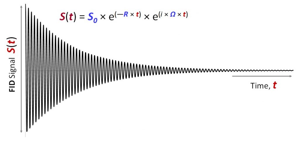
Figure V.3.A above shows a typical shape of the FID signal (current) vs. time: it is a harmonically oscillating, exponentially decaying curve. The signal intensity depends on time approximately as follows:

Equation V.3.\ref{EQ:fd2}

\[\begin{eqnarray}S(t) &=& S _0 \cdot e ^{ -R \cdot t} \cdot e ^{i \cdot \Omega \cdot t}\label{EQ:fd2}\end{eqnarray}\]

Such a signal would be produced by a single type of a spin-½ nucleus, that is by a specific proton in our sample biomolecule (e.g. by ¹H_α of Pro108, or ¹³C_β in Ala35 etc.). Parameter Ω is the angular resonance frequency of this nucleus Ω = 2πν, where ν is the effective oscillatory frequency of this nucleus (ν_eff) described in Chapter V.2. Angular frequency Ω is often used in NMR theory for rather technical reasons, but essentially it is linear resonance frequency ν scaled by factor 2π. Parameter R in the equation above specifies the rate of relaxation from the excited state to thermal equilibrium forthis particular spin. Just like the resonance frequency Ω, relaxation rate R is specific to each nucleus as it depends on the local covalent and non-covalent environment of the nucleus (and not so much on the external magnetic field \(B_o\)). Lastly, factor S₀ corresponds to the initial signal (detected electric current) when time t=0. The value of S₀ depends on the amount of the sample and the spin-up vs spin-down population polarization, which in turn depends on the magnitude of the main magnetic field \(B_o\) and gyromagnetic ratio γ (mathematical details will come a bit later). The units of S and S₀ (they are the same as can be deduced from Equation V.3.1) usually do not play much role in practical use of NMR spectroscopy as we will see in later chapters. For clarity and simplicity, we can postulate here that S and S₀ have units of electric current: Ampere (Amp).

It is important to appreciate that relaxation rate R is measured in units of Hz. Because R does not depend on the external magnetic field strength \(B_o\) (it is almost correct), expressing it in any units other than Hz (e.g. in ppm) really gives no benefit. Thus, we have an example of two types of quantities, R and Ω, which can both be expressed in units of Hz or ppm. Importantly, for only one quantity – resonance frequency Ω (or ν) – it is meaningful to express it in relative units (ppm) to normalize the quantity with respect to the magnet strength \(B_o\). This is why relaxation rates R almost always are listed in units of Hz.

Example \(\PageIndex{1}\)

Let us consider an NMR spectrometer with an 11.7 Tesla magnet (\(B_o\) = 11.7 T). If for two protons, H_ref (reference) and H_a (target sample), their resonance frequency values are measured as 500,010,000 Hz and 500,000,000 Hz respectively, what are the chemical shift values in ppm (δ_ref and δ_a) ?

Solution

According to Equation V.3.1 above:

δ_ref = ( 500,010,000 {Hz} – 500,010,000 {Hz} ) / ( 500,010,000 {Hz} ) × 10⁶ ({ppm}) = 0 ppm (this makes sense: chemical shift of a reference is zero)

δ_a = ( 500,010,000 {Hz} – 500,000,000 {Hz} ) / ( 500,010,000 {Hz} ) × 10⁶ ({ppm}) = 20 ppm

The difference between the resonance frequencies of the reference and proton H_a are 20 ppm (this value is independent of magnet strength \(B_o\)) and 10,000 Hz (this value is proportional to \(B_o\) and thus will change proportionately to \(B_o\) if a different magnet is used for recording).

Example \(\PageIndex{2}\)

If we have two non-interacting (e.g., remotely placed) spin-½ nuclei a and b within the sample molecule, each can generate an NMR signal described by formula 5.3.2 above, S_a(t) and S_b(t) respectively. How would a combined signal generated by the entire molecule can be mathematically described?

Solution

S(t) = S_a(t) + S_b(t)

Practice Problems

Problem 1. Consider Example 1 above. Calculate the chemical shift of proton H_A and reference proton H_ref as well as the chemical shift difference if the same recording is done on a magnet with: a) \(B_o\)= 9.4 Tesla, b) \(B_o\) = 23.4 Tesla. Calculate all the values in units of both Hz and ppm and compare the obtained numbers with the results of Example 1 above.

Problem 2. Example 1 above shows how to calculate chemical shift δ in units of ppm using oscillatory resonance frequency ν. Will the value δ change if instead oscillatory frequency one uses angular frequency \(\omega\) and if yes, what will the difference be?.

Problem 3. Let’s consider two spin-½ nuclei: nucleus a having relaxation rate R_a=10 Hz, the other, nucleus b, having relaxation rate R_b = 100 Hz. Which signal, the one from nucleus a or the one from nucleus b, will be reduced faster below 10% of their initial values, S_0a and S_0b respectively? Justify quantitatively.

Problem 4. Let’s consider two spin-½ nuclei described in Example 1 above. What nucleus, H_ref or H_a, will give more oscillations per unit of time when their NMR signals, S_ref(t) and S_a(t) respectively, are recorded and analyzed? Justify quantitatively.

Problem 5*. Imagine that both axes on Figure V.3.1 are labeled with actual numbers. Can you determine the numerical value of the resonance frequency Ω from this graph? If so, describe the algorithm for such a determination.