5.1: Nuclear Spin and Magnetic Field

In this Chapter, we will discuss why certain types of atomic nuclei are sensitive to the external magnetic field due to their quantum property known as the “spin”. We further will cover the dependence between the magnetic sensitivity of atomic nuclei and quantization of their energy levels once these atoms are exposed to the magnetic fields. After completing this Chapter, you will be able to quantitatively determine the frequency of magnetic resonance of a specific type of atomic nucleus exposed to a magnetic filed of certain strength.

Learning Objectives

• Understand the connection between nuclear quantum spin and nuclear magnetic moment
• Grasp the effect of external magnetic field on the quantization of nuclear spin energy levels (Zeeman split)
• Develop appreciation of the dependence of the resonance nuclear frequency on the strength of the magnetic field.

Nuclear “Spin”

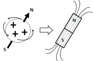
Atomic nucleus is a particle of subatomic scale. Thus, it can be described by a set of “quantum properties”. One of them is called “nuclear spin”, which fundamentally is related to the sensitivity of the nucleus to the effects of external magnetic fields (Figure V.I.A). In some sense (which is an oversimplification), an atomic nucleus with a non-zero spin value can be viewed as a little magnet, sensitive to the presence of an external magnetic field.

Figure V.I.A Non-zero nuclear “spin” provides a “quantum magnetic moment” to the atomic nucleus.

The nuclear spin value depends on the proton/neutron composition of the nucleus the atom or isotope. Table V.I.I lists some examples of nuclei with spin values of 0, ½, and 1 (the table does not include examples of spin values above 1):

Table V.1.I

Spin	Relevant Isotopes	Common features of the nuclei/isotopes
0	^12C, ^16O	Nuclei composed of even numbers of protons and even numbers of neutrons
½	^1H, ^13C, ^15N, ^31P, ^19F, ^129Xe	Nuclei composed of odd number of nucleons (protons and neutrons)
1	^2H, ^14N	Nuclei composed of odd numbers of protons and odd numbers of neutrons

Zeeman Splitting of Spin-½ Nuclei

In this textbook, we will almost exclusively consider the spin-½ nuclei and their interactions with external magnetic fields. Such interactions are at the heart of Nuclear Magnetic Resonance (NMR) spectroscopy, a central experimental method according to the classification of the American Chemical Society. As we will see in this and next chapters, modern NMR spectroscopy is widely utilized to address many problems in biochemistry, biophysics and other areas of life sciences in general. Figure V.I.B shows a modern NMR spectroscopy system and its central components: the superconducting magnet with the probe (where the sample in an NMR tube is subjected to external magnetic fields) and consoleor spectrometer (an elaborate assembly of advanced electronics circuits collectively controlling the process of magnetic field application and data recording).

Figure V.I.B A modern NMR spectrometer: Bruker Avance III HD (a cabinet on the background) equipped with a 16.4 Tesla (700 MHz, ¹H frequency) superconducting magnet (a large cylinder on three vibration-canceling suspension legs).

Under an external magnetic field \(B_o\), the energy E(m) of a quantum particle with a spin projection \(m\) on the axis of \(B_o\) (magnetic field is a vector!) is given by the following formula:

Equation V.1.\ref{EQ:se1}

\[\begin{eqnarray}E(m) &=& -m \cdot h \cdot \gamma \cdot B _0\label{EQ:se1}\end{eqnarray}\]

In the formula above, \(m\) denotes quantized spin projection value on the axis of \(B_o\): only \(m\) values of +½ and -½ are possible for spin-½ nuclei. Next, h denotes Plank's constant, which we first introduced in Chapter IV.3. The value of γ is specific to each isotope type, with \(\gamma\) values for some spin-½ isotopes listed in Table V.I.II.

Table V.1.II

Spin-½ Nucleus	^1H	^19F	^31P	^129Xe	^13C	^15N
γ, MHz/Tesla	42.58	40.05	17.24	-11.78	10.71	-4.32
|γ| relative to ^1H	1.0	0.94	0.40	0.28	0.25	0.10

Because only two spin projection values (½ and -½) are possible for spin-½ nuclei, formula (1) above tells that only two states (projections on \(B_o\)) with their respective two energy levels E(½) , E(-½) and energy difference (split) ΔE = E(-½) – E(½) are possible for such spins placed in an external magnetic field \(B_o\):

Equation \ref{EQ:se2}

\[\begin{eqnarray}E (1/2) &=& – \frac {1}{2} \cdot h \cdot \gamma \cdot B _0 \\[4pt] E (-1/2) &=& \frac {1}{2} \cdot h \cdot \gamma \cdot B _0 \\[4pt] \Delta E &=& h \cdot \gamma \cdot B _0\label{EQ:se2}\end{eqnarray}\]

A Split Spin-½ System and Nuclear Magnetic Resonance effect

Thus, a population of spin-½ particles will split into two sub-populations N(½) and N(-½) with their respective energy levels: lower value E(½) and higher value E(-½). At thermal equilibrium, the respective values of N(½) and N(-½) will be related via the Boltzmann distribution (covered in Chapter I.5):

Equation V.1.\ref{EQ:zs3}

\[\begin{eqnarray}\frac{N(-1/2)}{N(1/2)} &=& e^{-\frac{\Delta E}{k _B \cdot T}}\label{EQ:zs3}\end{eqnarray}\]

Equation V.1.\ref{EQ:zr3}

\[\begin{eqnarray}\frac{N(-1/2)}{N(1/2)} &=& e^{-\frac{h \cdot \gamma \cdot B_0}{k_B \cdot T}}\label{EQ:zr3}\end{eqnarray}\]

Such a separation into two sub-population of a nuclear spin-½ system under an external magnetic field \(B_o\) is called the Zeeman splitting. This split, equilibrated system of spin-½ nuclei can be perturbed out of equilibrium by an energy quanta whose frequency corresponds to the ΔE value (resonance excitation). After the system is perturbed in this way, it can be allowed to relax back to the thermal equilibrium (Boltzmann distribution) and the energy emitted during relaxation can be detected. Energy required to excite a nuclear spin-½ system and energy detected during relaxation of the excited system constitute the essence of Nuclear Magnetic Resonance (NMR) effect.

Example \(\PageIndex{1}\)

Let’s calculate the value of the Zeeman energy splitting ΔE for protons (¹H) under an external magnetic field B₀ = 11.7 Tesla (as in eq. (2) above):

Solution

ΔE = 6.626 × 10^-34 {J/Hz} × 42.58 {MHz/Tesla} × 10⁶ {Hz} / 1 {MHz} × 11.7 {Tesla} = 3.30 × 10^-25 J

Practice Problems

Problem 1. List at least four types of atoms/isotopes whose nuclei have spin-½ properties.

Problem 2. Calculate ΔE value (Zeeman split) in units of Joules for each of the spin-½ nuclei listed in Table V.1.II above in an external magnetic field \(B_o\) of 11.7 Tesla. What is the effect of the gyromagnetic ratio γ on the value of ΔE ?

Problem 3. Explore the effect of the strength of the external magnetic field value \(B_o\) on the value of the Zeeman energy split ΔE by doing problem 2 above at \(B_o\) = 23.4 Tesla.

Problem 4. The term γ⋅\(B_o\) appears in equations (1), (2) and (3) above and will appear in several key formulas later. What are the units of this product γ⋅\(B_o\)? What does this observation tell you about the physical meaning of γ⋅\(B_o\) (what processes it might represent)? Take a note of it as it will become relevant in the next chapter.

Problem 5. Compare the nuclear spin-½ Zeeman energy splitting (ΔE) value calculated in the Examples above with the electron energy level gap corresponding to UV irradiation of λ=280 nm. Which energy gap is greater: the one for a ¹H system at \(B_o\)=11.7 Tesla or the one corresponding to UV light of λ=280 nm?