3.1: Potential Energy Surface and Bonding Interactions

In this chapter, we return to the idea of a potential energy surface and consider models for a covalent bond. The potential energy changes as a function of the relative distance between bonded atoms. As atoms come together to form molecules, the potential energy will have a minimum at the equilibrium bond distance. For diatomic molecules, the potential energy surface is one-dimensional and depends only on the distance between the two atoms in the diatomic molecule. For polyatomic molecules with more complex structure, the potential energy surface will be a high-dimensional function of the positions all the atoms. To model the secondary structure of proteins and other macromolecules, we need potential energy functions to describe the equilibrium bond stretching of covalent bonds, the equilibrium angle bending (involving an angle between three atoms), and dihedral torsional rotations (involving four atoms). In this chapter we will look at empirical potential energy functions for these three type of interactions that govern the conformational energy of a polypeptide chain.

Learning Objectives

• Understand the difference between a harmonic potential energy and the Morse potential, and what is meant by the terms harmonic or anharmonic vibrations.
• Be able to explain and justify the different parameters used to describe single, double, and triple bonds.
• Be able to sketch the dihedral potential energy for the butane molecule.
• Understand the physical justification for the different types of empirical potential energy functions that describe bonding interactions.

The chemical bond

The starting place for understanding chemical bonding and molecular structure is the Born Oppenheimer approximation. Since atomic nuclei are much heavier than the electrons, the electrons move much faster than the nuclei. Thus, to a good approximation, the motion of the atomic nuclei and electrons can be treated separately. The energy due to the electrons in the ground state can be calculated assuming a fixed position of the nuclei. This calculation can be repeated at different values of the internuclear distance between the atoms. This gives the potential energy for the nuclear positions as a function of the internuclear distance. As a consequence of the Born Oppenheimer approximation, we can think of the atomic nuclei as moving along a potential energy surface that is a function only of the nuclei position.

We begin by considering the simplest case of the potential energy curve for a diatomic molecule, such as H₂ that was introduced in Chapter II.3 in the context of transition state theory. Figure III.1.A again shows the potential energy curve for the H₂ molecule. Notice that the equilibrium bond length, labeled \(r_e\), is located at the minimum of the bond potential energy curve.

Figure III.1.A. Potential energy surface for molecular hydrogen as a function of the internuclear distance. The equilibrium bond distance corresponds to the minimum on the potential energy surface.

If the displacement away from the equilibrium bond length is small, the potential energy surface in the vicinity of the equilibrium bond distance can be described by a harmonic oscillator (see Appendix for the derivation)

\[V=\frac{1}{2}k \left(r-r_e\right)^2\label{EQ:harmonic_bond}\]

In Equation \ref{EQ:harmonic_bond}, \(r\) is the distance between the two atoms and \(r_e\) is the equilibrium bond distance. Figure III.1.B compares the full potential energy curve for H₂ with Equation \ref{EQ:harmonic_bond}. Notice that at sufficiently small displacements from \(r_e\), vibrations in the bond are accurately described by Equation \ref{EQ:harmonic_bond}. Oscillations that are described by Equation \ref{EQ:harmonic_bond} are called harmonic. In a harmonic bond, the force that results from stretching or compressing the bond distance is proportional to the displacement from the equilibrium position (Hook’s law).

\[\begin{eqnarray}\text{Force} &=& – \frac{dV}{dr} \\[4pt] &=& – k \left(r-r_e\right)\label{EQ:harmonic_force}\end{eqnarray}\]

Figure III.1.B. Comparison between Harmonic bond approximation (Equation \ref{EQ:harmonic_bond}) with the exact potential energy surface. The harmonic approximation is valid for small displacements from the equilibrium bond distance.

Equations III.1.\ref{EQ:harmonic_bond} and III.1.\ref{EQ:harmonic_force} describe small perturbative fluctuations about the equilibrium bond distance. In this case, the bonds are said to be harmonic bonds. Large displacements of the bond away from \(r_e\) lead to anharmonic vibrations. Anharmonic vibrations describe bond stretching that is far from the equilibrium bond distance. To model anharmonic vibrations, we could consider including higher-order terms in the Taylor expansion in Appendix. Alternatively, a common potential that can model bond breaking is the Morse potential:

\[V = D_e \left(1 – e^{-a (r-r_e)}\right)^2 \label{EQ:harmonic_bond2}\]

where \(D_e\) is the bond dissociation energy, and \(a\) controls the potential width. Figure III.1.C shows a plot of the Morse potential.

Figure III.1.C. To a good approximation anharmonic bond vibrations can be modeled using the Morse potential given by Equation \ref{EQ:harmonic_bond2}. Figure III.1.C show the Morse potential using parameters for the H₂ molecule.

The potential energy surface for macromolecules is high-dimensional

In the previous section we described the potential energy for a diatomic molecule, such as H₂, O₂, N₂, NO, etc …, in terms of the equilibrium bond distance \(\bf{r_e}\) and the internuclear distance \(\bf{r}\). As we saw in Chapter II.3 (see Figure II.3.C), for polyatomic molecules involving more than two bonded atoms, the potential energy surface is a function of all the internuclear distances and quickly becomes high-dimensional. For a proteins, nucleic acids, lipids, polysaccharides, or other macromolecules, if we let \(\textbf{R}\) be the set of positions of all the atoms ( \( \textbf{R}=\{\textbf{R}_1,\textbf{R}_2, …,\textbf{R}_N \} \) ), then the potential energy surface \(U(\textbf{R})\) will be a function of all atomic coordinates. Although we cannot draw in more than three dimensions, we can consider an abstract high-dimensional space where a point is given by the set of all the atomic positions: \((\textbf{R}_1,\textbf{R}_2, …,\textbf{R}_N)\). Local minima in this high-dimensional space will represent metastable conformations and local maxima represent kinetic barriers.

At constant number of particles, temperature, and volume, the probability of a given conformation is given by the normalize Boltzmann weight of the energy:

\[P(\textbf{R}) = \frac{e^{-U(\textbf{R})/k_BT}}{\int ... \int e^{-U(\textbf{R})/k_BT} \ d\textbf{R}_1, ..., d\textbf{R}_N}\label{EQ:Boltzman}\]

where the integral in the denominator is a multi-dimensional integral over all the atomic coordinates. It is common practice in computational biophysics to reduce the high-dimensional potential energy landscape to a limited number of variable that can describe the conformational state of the system, called order parameters or collective variables. An example of this was already present in Chapter II.3 where we reduce the two-dimensional potential energy surface for the S_N2 substitution to a one-dimensional picture by constructing a path along the lowest energy contour from the reactant to product state as shown in Figure III.1.D

Figure III.1.D. The "high dimensional" representation of the potential energy surface for the S_N2 reaction as a function of the C-Cl bond distance and C-Br bond distance. A "low dimensional" representation along the hypothetical reaction coordinate is shown on the right along the red curve corresponding to the lowest energy path between reactant and product states. The transition state is the highest energy intermediate state between the reactant and product along the reaction coordinate.

As another example, we can consider the two dihedral angels, \(\phi\) and \(\psi\) for the Nme-Ala-Ace peptide shown here:

Figure III.1.E. Two metastable states of the Nme-Ala-Ace peptide are characterized by the two Ramachandran dihedral angles, \(\phi\) and \(\psi\).

Imagine we could sample randomly the equilibrium configurations drawn from a Boltzmann distribution of states given by Equation \ref{EQ:Boltzman}. In this case, we could construct a histogram of all \(\phi\), \(\psi\) angle combinations to obtain the probability \(P(\phi, \psi)\). From statistical biophysics, we can define a free energy surface from the probabilities as

\[F(\phi,\psi) = -k_BT \ln P(\phi,\psi) \label{EQ:FES}\]

The free energy surface is a low-dimensional representation of system that provides information about metastable states, their relative stability, and the free energy barriers separating them. An example two-dimensional free energy surface for the Nme-Ala-Ace peptide is shown in Figure III.1.F. From this surface, we can define the transition state as the separatrix where there is equal probability for the system to flow into either metastable basin.

Figure III.1.F. The two-dimensional free energy surface for the Nme-Ala-Ace peptide projected on the space of the two Ramachandran dihedral angles, \(\phi\) and \(\psi\). The transition state is defined as the separatrix where there is equal probability for the system to flow into either metastable basin.

The covalent bond revisited

In molecular mechanics, we are often interested in equilibrium fluctuations of chemical bonds. For small fluctuations, it is customary to use a harmonic potential for the form of \ref{EQ:X}:

\[V=\frac{1}{2}k \left(r-r_e\right)^2 \label{EQ:X}\]

The spring constant \(k\) determines the stiffness of the bond and the value of \(r_e\) is the equilibrium bond distance. These values are parameters of the model and are usually empirically determined to fit to experimentally observed values (for example from IR spectroscopy). Each type of chemical bond will need to be parameterized to agree with experiment. For example, a carbon-carbon single bond, between two sp³ carbon atoms, such as in the ethane molecule shown in Figure III.1.G (a) will have a slightly larger value of \(r_e\) and a slightly smaller value of \(k\) as compared to a carbon-carbon double bond, between two sp² carbon atoms, such as in the ethene molecule shown in Figure III.1.G (b).

Figure III.1.G. The single bond between the sp³ hybridized carbons in the ethane molecule (a) has a longer equilibrium bond length and is weaker than the double bond between the sp² hybridized carbons in the ethene molecule (b). As a result the parameters in the harmonic bond potential energy function will be different for different hybridizations of carbon.

Table III.1.a shows the values for the spring constant and equilibrium bond distance for the different bond orders of carbon bonds.

hybridization	bond order	spring constant, k	equilibrium bond distance, re
sp^3	1	100 kcal/mol/Å^2	1.5 Å
sp^2	2	200 kcal/mol/Å^2	1.3 Å
sp	3	400 kcal/mol/Å^2	1.2 Å

Figure III.1.H shows a plot of the harmonic bond for each type of bond (single, double, and triple). We can see that as the bond order increases, the equilibrium bond distance, \(r_e\), decreases, and the stiffness of the bond, \(k\) increases.

Figure III.1.H. The potential energy function of a carbon-carbon single bond (sp³ hybridization) vs. a carbon-carbon double bond (sp² hybridization) vs. a carbon-carbon triple bond (sp hybridization). The parameters for each bond type are given in Table III.1.a

Angular and dihedral potentials for polyatomic molecules

In molecules with more than two bonded atoms it is possible to define a bond angle shown in Figure III.1.I. A bond angle is formed by three consecutive atoms, here labeled \(i\), \(j\), and \(k\). The corresponding bond angle is \(\theta\). If we let \(\textbf{r}_{ij}\) be the bond distance between atoms \(i\) and \(j\) and \(\textbf{r}_{jk}\) the bond distance between atoms \(j\) and \(k\), the bond angle can be expressed in terms of the atomic positions as

\[\theta = \arccos \left(\frac{\textbf{r}_{ij}\cdot \textbf{r}_{jk}}{|r_{ij}||r_{jk}|} \right)\label{EQ:Bondangle}\]

where the dot indicates the dot product between bond vectors \(\textbf{r}_{ij}\) and \(\textbf{r}_{jk}\) and \(|r_{ij}|\) and \(|r_{jk}|\) are the lengths of the bond vectors.

It is common to describe fluctuations about the equilibrium bond angle with a harmonic potential of the form:

\[V_{angle} =\frac{1}{2}k \left(\theta-\theta_e\right)^2\label{EQ:angle}\]

where \(\theta_e\) is the equilibrium bond angle and \(k\) is a force constant that parameterizes the stiffness of the bond angle.

Figure III.1.I. Fluctuations about the equilibrium bond angle, \(\theta\), can be modeled using a harmonic potential energy function about the equilibrium bond angle \(\theta_e\).

If we are interested in the force acting on atom \(i\), as we would need for solving Newton’s equation of motion, we can use the chain rule:

\[\frac{dV}{d r_i} = \frac{dV}{d\theta}\cdot \frac{d\theta}{d r_i}\label{EQ:chainrule}\]

where the derivate \(\frac{dV}{d\theta}\) can be computed by taking the derivative of Equation \ref{EQ:angle} with respect to \(\theta\), and the derivative \(\frac{d\theta}{d r_i}\) can be computed by taking the derivative of Equation \ref{EQ:Bondangle} with respect to \(r_i\).

For atoms with four or more bonded atoms, there is a potential energy barrier to internal rotation about the dihedral angles. As a simple example we will consider the rotation about the methyl dihedral in butane as shown below:

The lowest energy configuration is the staggered, anti-, geometry at a bond angle of 180º. There are two equivalent staggered configurations with bond angles of 300º and 60º which are 3.8 kJ mol^-1 higher in energy. The large energy barrier of 19 kJ mol^-1 for the eclipsed, sys-, geometry means that rotations from on gauche configuration (300º) into another gauche configuration (60º) will be a rare event. To model a periodic potential energy function as seen in Figure III.1.J, the torsional energy is given by:

\[V_{torsion} = A[1 + \cos (n \phi – \phi_0)]\label{EQ:torsion}\]

where \(\phi\) is the dihedral angle of interest and the parameter \(A\) is a constant with units of energy, \(n\) is an integer, and \(\phi_0\) is a reference dihedral angle.

Figure III.1.J. The dihderal potential energy about the methyl bond in the butane molecule that can be modeled by Equation \ref{EQ:torsion}. The potential energy function has a period of 360º with the lowest energy configuration in the staggered, anti, configuration with a bond angle of 180º. The maximum in energy occurs at for the eclipsed configuration with a bond angle of 0º.

As an example, consider the the structure of the retinal chromophore shown in Figure III.1.K which has a conjugated \(\pi\) bond system. Absorption of a photon induces an excited state of the chromophore which is followed by the isomerization of the retinal protonated Schiff base around the C₁₃=C₁₄ bond (adjacent to the Schiff base group). Rotation of the dihedral bonds can be modeled using Equation \ref{EQ:torsion}. Table III.1.b reports the parameter set used in molecular dynamics simulations of the retinal Schiff base.

Figure III.1.K. Structure of retinal chromophore covalently bound to Lys216. Photoisomerization leads to rotation of the dihedral angle about the C₁₃=C₁₄ bond

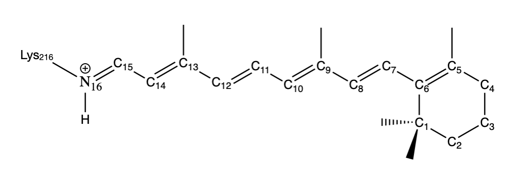
Table III.1.b. The parameter set for the torsion potentials of the main polyene chain of the retinal Schiff base. Values taken from Tajkhorshid et al. 1999. The form of the torsion potential is given by Equation \ref{EQ:torsion}.

\(\phi \)	\(A \) kcal/mol	\(n\)	\( \phi_0 \) (degrees)
C5-C6-C7-C8	5.62	2.0	180.0
C6-C7-C8-C9	19.99	2.0	180.0
C7-C8-C9-C10	8.515	2.0	180.0
C8-C9-C10-C11	18.64	2.0	180.0
C9-C10-C11-C12	11.25	2.0	180.0
C10-C11-C12-C13	17.54	2.0	180.0
C11-C12-C13-C14	14.15	2.0	180.0
C12-C13-C14-C15	14.73	2.0	180.0
C13-C14-C15-N16	15.215	2.0	180.0
C14-C15-N16-C\(_\epsilon\)	14.38	2.0	180.0

Practice Problems

Coming soon ...