16.7: Weak Bases

The pH of a solution of a weak base can be calculated in a way which is very similar to that used for a weak acid. Instead of an acid constant K_a, a base constant K_b must be used. If a weak base B accepts protons from water according to the equation

\[\text{B} + \text{ H}_{\text{2}}\text{O}\rightleftharpoons\text{BH}^{+} + \text{OH}^{-} \label{1} \]

then the base constant is defined by the expression

\[K_{b}=\dfrac{ \text{ BH}^{\text{+}} \text{ OH}^{-} }{ \text{ B } } \label{2} \]

A list of K_b values for selected bases arranged in order of strength is given in the table below. This table is part of our larger collection of acid-base resources. 

Table \(\PageIndex{1}\): The Base Constants for Some Bases at 25°C. Taken from Hogfelt, E. Perrin, D. D. Stability Constants of Metal Ion Complexes, 1^st ed. Oxford; New Pergamon, 1979-1982. International Union of Pure and Applied Chemistry, Commission on Equilibrium. ISBN: 0080209580

Base	Formula and Ionization Equation	Kb	Molecular Shape
Ammonia	\(NH_3 + H_2O \rightleftharpoons NH^+_4 + OH^–\)	1.77 × 10^–5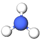
Aniline	\(C_6H_5NH_2 + H_2O \rightleftharpoons C_6H_5NH^+_3 + OH^–\)	3.9 × 10^–10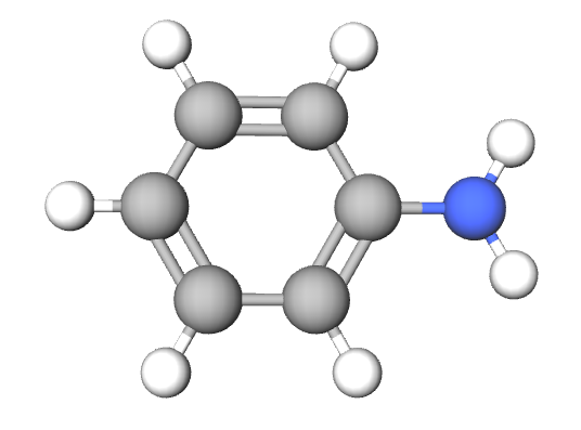
Carbonate ion	\(CO_3^{2–} + H_2O \rightleftharpoons HCO^-_3 + OH^–\)	2.1 × 10^–4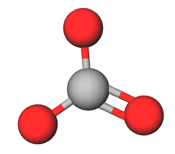
Hydrazine	\(N_2H_4 + H_2O \rightleftharpoons N_2H^+_5 + OH^–\) \(N_2H^+_5 + H_2O \rightleftharpoons N_2H_6^{2+} + OH^–\)	K1 = 1.2 × 10^–6 K2 = 1.3 × 10^–15
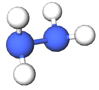Hydride ion	\(H^– + H_2O \rightarrow H_2 + OH^–\)	1.0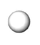
Phosphate ion	\(PO_4^{3–} + H_2O \rightleftharpoons HPO^{2-}_4 + OH^–\)	5.9 × 10^–3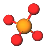
Pyridine	\(C_5H_5N + H_2O \rightleftharpoons C_5H_5NH^+ + OH^–\)	1.6 × 10^–9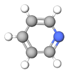

To find the pH we follow the same general procedure as in the case of a weak acid. If the stoichiometric concentration of the base is indicated by c_b, the result is entirely analogous to equation 4 in the section on the pH of weak acids; namely,

\[K_{b}=\dfrac{ [\text{OH}^{-}]^2}{c_{b}- [\text{ OH}^{-}] } \label{3} \]

Under most circumstances we can make the approximation

\[c_b – [OH^–] \approx c_b \nonumber \]

in which case Equation \ref{3} reduces to the approximation

\[[OH^–] ≈ \sqrt{K_{b}c_{b}} \label{4} \]

which is identical to the expression obtained in the acid case (approximation shown in equation 6 in the section on the pH of weak acids) except that OH^– replaces H₃O⁺ and b replaces a. Once we have found the hydroxide-ion concentration from this approximation, we can then easily find the pOH, and from it the pH.

Example \(\PageIndex{1}\): pH using K_b

Using the value for K_b listed in the table, find the pH of 0.100 M NH₃.

Solution

It is not a bad idea to guess an approximate pH before embarking on the calculation. Since we have a dilute solution of a weak base, we expect the solution to be only mildly basic. A pH of 13 or 14 would be too basic, while a pH of 8 or 9 is too close to neutral. A pH of 10 or 11 seems reasonable. Using Equation \ref{4} we have

\[\begin{align*} [\text{ OH}^{-}] &=\sqrt{K_{b}c_{b}} \\[4pt] & =\sqrt{\text{1.8 }\times \text{ 10}^{-\text{5}}\text{ mol L}^{-\text{1}} \times \text{ 0.100 mol L}^{-\text{1}}} \\[4pt] &=\sqrt{\text{1.8 }\times \text{ 10}^{-\text{6}}\text{ mol}^{\text{2}}\text{ L}^{-2}} \\[4pt] &=\text{1.34 }\times \text{ 10}^{-\text{3}}\text{ mol L}^{-\text{1}} \end{align*} \nonumber \]

Checking the accuracy of the approximation, we find

\(\dfrac{ [\text{ OH}^{-} ]}{c_{\text{b}}}=\dfrac{\text{1.34 }\times \text{ 10}^{-\text{3}}}{\text{0.1}}\approx \text{1 percent}\)

The approximation is valid, and we thus proceed to find the pOH.

\(\text{pOH}=-\text{log}\dfrac{ [\text{ OH}^{-} ]}{\text{mol L}^{-\text{1}}}=-\text{log(1.34 }\times \text{ 10}^{-\text{3}}\text{)}=\text{2.87}\)

From which

\[pH = 14.00 – pOH = 14.00 – 2.87 = 11.13 \nonumber \]

This calculated value checks well with our initial guess. 

Occasionally we will find that the approximation 

\[c_b – [OH^{–}] ≈ c_b \nonumber \]

is not valid, in which case we must use a series of successive approximations similar to that outlined above for acids. The appropriate formula can be derived from Equation \ref{3} and reads

\[[OH^{-}] \approx \sqrt{K_{b} ( c_b - [OH^{-}] )} \nonumber \]