1.5: Polymer Chemistry

All measurements have a degree of uncertainty regardless of precision and accuracy. This is caused by two factors, the limitation of the measuring instrument (systematic error) and the skill of the experimenter making the measurements (random error).

Introduction

The graduated buret in Figure 1 contains a certain amount of water (with yellow dye) to be measured. The amount of water is somewhere between 19 ml and 20 ml according to the marked lines. By checking to see where the bottom of the meniscus lies, referencing the ten smaller lines, the amount of water lies between 19.8 ml and 20 ml. The next step is to estimate the uncertainty between 19.8 ml and 20 ml. Making an approximate guess, the level is less than 20 ml, but greater than 19.8 ml. We then report that the measured amount is approximately 19.9 ml. The graduated cylinder itself may be distorted such that the graduation marks contain inaccuracies providing readings slightly different from the actual volume of liquid present.

 

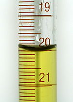
Figure 1: A meniscus as seen in a burette of colored water. '20.00 mL' is the correct depth measurement. Click here for a more complete description on buret use, including proper reading. Figure used with permission from Wikipedia.

Systematic vs. Random Error

The diagram below illustrates the distinction between systematic and random errors.

Figure 2: Systematic and random errors. Figure used with permission from David DiBiase (Penn State U).

 

Systematic errors: When we use tools meant for measurement, we assume that they are correct and accurate, however measuring tools are not always right. In fact, they have errors that naturally occur called systematic errors. Systematic errors tend to be consistent in magnitude and/or direction. If the magnitude and direction of the error is known, accuracy can be improved by additive or proportional corrections. Additive correction involves adding or subtracting a constant adjustment factor to each measurement; proportional correction involves multiplying the measurement(s) by a constant.

Random errors: Sometimes called human error, random error is determined by the experimenter's skill or ability to perform the experiment and read scientific measurements. These errors are random since the results yielded may be too high or low. Often random error determines the precision of the experiment or limits the precision. For example, if we were to time a revolution of a steadily rotating turnable, the random error would be the reaction time. Our reaction time would vary due to a delay in starting (an underestimate of the actual result) or a delay in stopping (an overestimate of the actual result). Unlike systematic errors, random errors vary in magnitude and direction. It is possible to calculate the average of a set of measured positions, however, and that average is likely to be more accurate than most of the measurements.

Note

Systematic and random errors refer to problems associated with making measurements. Mistakes made in the calculations or in reading the instrument are not considered in error analysis. It is assumed that the experimenters are careful and competent!

A Graphical Representation

In this experiment a series of shots is fired at a target. Random errors are caused by anything that makes the shots inconsistent and arrive at the target at random different points. For example, the shooter has an unsteady hand or a change in the environment may distort the shooter's view. These errors would result in the scattering of shots shown by the right target in the figures to the left. A systematic error, on the other hand, would include consistent errors that always arise. For example, the gun may be misaligned or there may be some other type of technical problem with the gun. This type of error would yield a pattern similar to the left target with shots deviating roughly the same amount from the center area.

When measuring a defined length with a ruler, there is a source of uncertainty and the measurement may need estimation or rounding between two points. When doing this estimation, it is possible to over estimate and under estimate the measured value, meaning there is a possibility for random error. Also, the ruler itself may be too short or too long causing a systematic error. For example, the illustration to the right shows a pencil whose length lies between 25 cm and 26 cm. With an intermediate mark, the ruler shows in greater detail that the pencil length lies somewhere between 25.5 cm and 26 cm. Therefore, one may reasonably approximate that the length of the pencil is 25.7 cm. The presence of a systematic error, however, would likely be more subtle than a random error because the environment may affect the ruler in a difficult to notice way or the ruler itself may have slightly inaccurate markers.

Figure 3: Systemic Error in length measurements via ruler.

Precision vs. Accuracy

Precision is often referred to as reproducibility or repeatability. For example, consider the precision with which the golf balls are shot in the figures below. A set of shots that are only precise would mean you are able to cluster your shots near each other on the green but you are not reaching your goal, which would be to get the golf balls into the hole. This concept is illustrated in the left picture of the two figures below. Accuracy, on the other hand, is how close a value is to the true or accepted value. The picture to the right demonstrates accuracy showing that the balls all get into the hypothetically large hole but are all at different corners of the hole. Therefore, the shots are not precise since they are relatively spread out but they are accurate because they all reached the hole. To sum up this concept, accuracy is the ability to hit the desired target area or measured value while precision is the agreement of shots or measured values with each other but not with the intended target or value.

Example 1

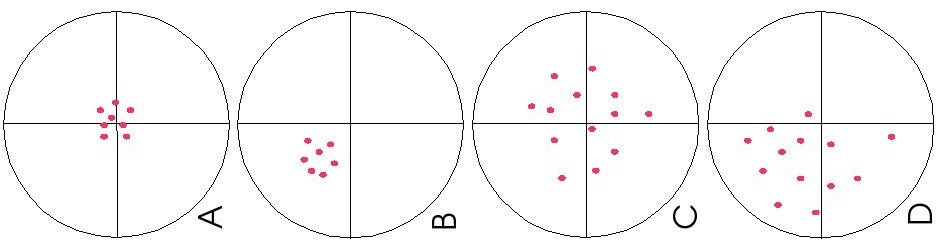
The following archery targets show marks that represent the results of four sets of measurements. Which target shows

1. a precise but inaccurate set of measurements?
2. an accurate but imprecise set of measurements?
3. a set of measurements that is both precise and accurate?
4. a set of measurements that is neither precise nor accurate?

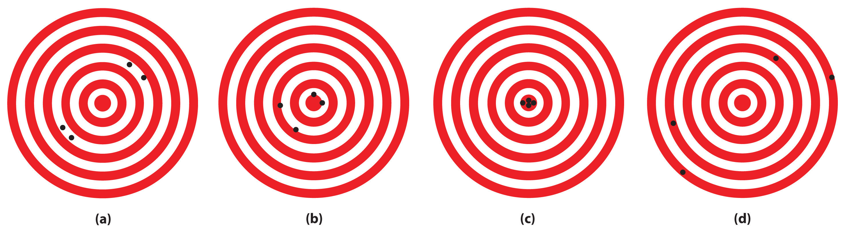
SOLUTION

1. (B)
2. (a)
3. (c)
4. (d)

Calculating Error

Since equipment used in an experiment can only report a measured value with a certain degree of accuracy, calculating the extent to which a measurement deviates from the value accepted by the scientific community is often helpful in gaging the accuracy of equipment. Such a calculation is referred to as the percent error of a measurement and is represented by the following formula:

\[\text{Percent Error} = \dfrac{\text{Experimental Result - Accepted value}}{\text{Accepted Value}} \times 100\%\]

Example 2 is a real world example to understand the role of percent error calculations in determining the accuracy of measuring equipment.

Example 2

A toy company that ships its products around the world must calculate fuel costs associated with transporting the weight of their standard 2 by 3 foot box. To predict shipping costs and create a reasonable budget, the company must obtain accurate mass measurements of their boxes. The accepted mass of a standard box is 0.525 kg. The company measures a sample of three dozen boxes with a sophisticated electronic scale and an analog scale each yielding an average mass of 0.531 kg and 0.49 kg, respectively. A calculation of percent error for each device yields the following results:

Percent Error of Electronic Scale = [(0.531kg - 0.525kg) / 0.525kg] X 100% = 1.14 %

Percent Error of Analog Scale = [(0.49kg - 0.525kg) / 0.525kg] X100% = -6.67%

Immediately, one notices that the electronic scale yields a far more accurate measurement with a percent error almost six times lower than the measurement obtained from the analog scale. Also note that percent error may take on a negative value as illustrated by the calculation for the analog scale. This simply indicates that the measured average lies 6.67% below the accepted value. Conversely, a positive percent error indicates that the measured average is higher than the accepted value.

1.  

Methods of Reducing Error

While inaccuracies in measurement may arise from the systematic error of equipment or random error of the experimenter, there are methods that can be employed to reduce error:

Weighing by difference: Mass is an important measurement in many experiments and it is critical for labs to reduce error in mass measurements whenever possible. A simple way of reducing the systematic error of electronic balances commonly found in labs is to weigh masses by difference. This procedure entails the following:

1. finding the mass of both the desired material and the container holding the material,
2. transferring an approximate amount of the material to another container,
3. remeasuring the mass of the original container, and
4. calculating the mass of the removed sample by taking the difference between the initial and final weights of the original container. The following formula illustrates the procedure used for weighing by difference:

(mass of container + mass of material) - (mass of container + mass of material after removing material) = mass of removed material

While most electronic balances have a "tare" or "zero" function that allows one to automatically calculate a mass by difference, equipment can be faulty so it is important to remember the fundamental logic behind weighing by difference.

• Averaging Results: Since the accuracy of measurements are limited in part to the capacity of an experimenter to interpret their equipment, it makes sense that the average of several trials would be taken rather than a single trial. The reasoning behind averaging results is that an error of a measured value that falls below the actual value may be accounted for by averaging with an error that is above the actual value. By performing a series of trials (the more trials the more accurate the averaged result), an experimenter can account for some of their random error and yield a measurement with higher accuracy.
• Calibrating Equipment: Just as random error can be reduced by averaging several trials, systematic error of equipment can be reduced by calibrating a measuring device. This usually entails comparing a standard device of well known accuracy to the second device requiring calibration. Additionally, procedures exist for different kinds of equipment that can reduce the systematic error of the device. For example, a typical buret in a lab may be used to carry out a titration involving neutralization of an acid and base. If the buret formerly held acid but must now hold a base, then it would benefit the experimenter to condition the buret with the base before carrying out the titration so that the buret may acclimate to the new substance and provide a more accurate reading. Such procedures, together with calibration, can reduce the systematic error of a device.

References

1. Pettrucci, Ralph H. General Chemistry: Principles and Modern Applications. 9th. Upper Saddle River: Pearson Prentice Hall, 2007.
2. Taylor, John Robert. Introduction to Error Analysis: The Study of Uncertainties in Physical Measurements. University Science Books. p. 94, §4.1. ISBN 093570275X
3. Kotz, John C. Chemistry and Chemical Reactivity. 7th. Belmont, CA: Thomson Brooks/Cole, 2009.

Problems

1. Is it possible to be accurate but not precise?
2. When measuring a given amount of water from a cylinder, the cylinder itself has been distorted and many of the readings done need estimation by the experimenter. What is the random error, and what is the systematic error?
3. If a person were to approximate the volume of liquid in the following picture to be 43.1 ml, what type of error would their estimate be?

4. In a target practice, draw examples of: (A) precision and accuracy, (B) precise but not accurate, (C) accurate but not precise, and (D) neither
5. Tom conducted an experiment using the GENSYS-20 and his results were consistently off from the actual absorbance for the wavelength. Is this a systematic or random error?
6. Claire decided to time her dog lap times with a stop watch. Her results were varied after 10 trials. Why is this so?
7. A researcher measures the length of a particular steel bolt to be 24.35 cm. If the accepted value for the length of this steel bolt is 24.20 cm, what is the percent error of the researcher's measurement?
8. A spectrophotometer gives absorbance readings that are consistently higher than the actual absorbance of the materials being analyzed. What kind of systematic error is this?
9. An electronic balance lacks the ability to read a measured quantity as zero so researchers must weigh by difference to more accurately determine the mass of a material. What type of error is this inability to read zero called?
10. Susan measures the weight of a standard paper clip to be 0.97 grams. The accepted value for the mass of a paper clip is 1.05 grams. What is the percent error of Susan's measurement? Do you notice any peculiar differences between this percent error and the percent error found in problem 7?
11. If you had a beaker and some graphite how would you weigh the exact amount of graphite using the weighing of difference procedure?

Solutions

1. Yes, a series of measurements may all be close to the true or accepted value, but they can differ from each other making them imprecise.
2. The random error originates from the estimation required of the experimenter and the systematic error stems from distortions in the cylinder.
3. The approximation would be an example of random error.
4.  

5. Since Tom must rely on the machine for an absorbance reading and it provides consistently different measurements, this is an example of systematic error.
6. The majority of Claire's variation in time can likely be attributed to random error such as fatigue after multiple laps, inconsistency in swimming form, slightly off timing in starting and stopping the stop watch, or countless other small factors that alter lap times. To a much smaller extent, the stop watch itself may have errors in keeping time resulting in systematic error.
7. The researcher's percent error is about 0.62%.
8. This is known as multiplier or scale factor error.
9. This is called an offset or zero setting error.
10. Susan's percent error is -7.62%. This percent error is negative because the measured value falls below the accepted value. In problem 7, the percent error was positive because it was higher than the accepted value.
11. You would first weigh the beaker itself. After obtaining the weight, then you add the graphite in the beaker and weigh it. After obtaining this weight, you then subtract the weight of the graphite plus the beaker minus the weight of the beaker.