
1.9: The Heisenberg Uncertainty Principle
- Page ID
- 142951
\( \newcommand{\vecs}[1]{\overset { \scriptstyle \rightharpoonup} {\mathbf{#1}} } \)
\( \newcommand{\vecd}[1]{\overset{-\!-\!\rightharpoonup}{\vphantom{a}\smash {#1}}} \)
\( \newcommand{\id}{\mathrm{id}}\) \( \newcommand{\Span}{\mathrm{span}}\)
( \newcommand{\kernel}{\mathrm{null}\,}\) \( \newcommand{\range}{\mathrm{range}\,}\)
\( \newcommand{\RealPart}{\mathrm{Re}}\) \( \newcommand{\ImaginaryPart}{\mathrm{Im}}\)
\( \newcommand{\Argument}{\mathrm{Arg}}\) \( \newcommand{\norm}[1]{\| #1 \|}\)
\( \newcommand{\inner}[2]{\langle #1, #2 \rangle}\)
\( \newcommand{\Span}{\mathrm{span}}\)
\( \newcommand{\id}{\mathrm{id}}\)
\( \newcommand{\Span}{\mathrm{span}}\)
\( \newcommand{\kernel}{\mathrm{null}\,}\)
\( \newcommand{\range}{\mathrm{range}\,}\)
\( \newcommand{\RealPart}{\mathrm{Re}}\)
\( \newcommand{\ImaginaryPart}{\mathrm{Im}}\)
\( \newcommand{\Argument}{\mathrm{Arg}}\)
\( \newcommand{\norm}[1]{\| #1 \|}\)
\( \newcommand{\inner}[2]{\langle #1, #2 \rangle}\)
\( \newcommand{\Span}{\mathrm{span}}\) \( \newcommand{\AA}{\unicode[.8,0]{x212B}}\)
\( \newcommand{\vectorA}[1]{\vec{#1}} % arrow\)
\( \newcommand{\vectorAt}[1]{\vec{\text{#1}}} % arrow\)
\( \newcommand{\vectorB}[1]{\overset { \scriptstyle \rightharpoonup} {\mathbf{#1}} } \)
\( \newcommand{\vectorC}[1]{\textbf{#1}} \)
\( \newcommand{\vectorD}[1]{\overrightarrow{#1}} \)
\( \newcommand{\vectorDt}[1]{\overrightarrow{\text{#1}}} \)
\( \newcommand{\vectE}[1]{\overset{-\!-\!\rightharpoonup}{\vphantom{a}\smash{\mathbf {#1}}}} \)
\( \newcommand{\vecs}[1]{\overset { \scriptstyle \rightharpoonup} {\mathbf{#1}} } \)
\( \newcommand{\vecd}[1]{\overset{-\!-\!\rightharpoonup}{\vphantom{a}\smash {#1}}} \)
\(\newcommand{\avec}{\mathbf a}\) \(\newcommand{\bvec}{\mathbf b}\) \(\newcommand{\cvec}{\mathbf c}\) \(\newcommand{\dvec}{\mathbf d}\) \(\newcommand{\dtil}{\widetilde{\mathbf d}}\) \(\newcommand{\evec}{\mathbf e}\) \(\newcommand{\fvec}{\mathbf f}\) \(\newcommand{\nvec}{\mathbf n}\) \(\newcommand{\pvec}{\mathbf p}\) \(\newcommand{\qvec}{\mathbf q}\) \(\newcommand{\svec}{\mathbf s}\) \(\newcommand{\tvec}{\mathbf t}\) \(\newcommand{\uvec}{\mathbf u}\) \(\newcommand{\vvec}{\mathbf v}\) \(\newcommand{\wvec}{\mathbf w}\) \(\newcommand{\xvec}{\mathbf x}\) \(\newcommand{\yvec}{\mathbf y}\) \(\newcommand{\zvec}{\mathbf z}\) \(\newcommand{\rvec}{\mathbf r}\) \(\newcommand{\mvec}{\mathbf m}\) \(\newcommand{\zerovec}{\mathbf 0}\) \(\newcommand{\onevec}{\mathbf 1}\) \(\newcommand{\real}{\mathbb R}\) \(\newcommand{\twovec}[2]{\left[\begin{array}{r}#1 \\ #2 \end{array}\right]}\) \(\newcommand{\ctwovec}[2]{\left[\begin{array}{c}#1 \\ #2 \end{array}\right]}\) \(\newcommand{\threevec}[3]{\left[\begin{array}{r}#1 \\ #2 \\ #3 \end{array}\right]}\) \(\newcommand{\cthreevec}[3]{\left[\begin{array}{c}#1 \\ #2 \\ #3 \end{array}\right]}\) \(\newcommand{\fourvec}[4]{\left[\begin{array}{r}#1 \\ #2 \\ #3 \\ #4 \end{array}\right]}\) \(\newcommand{\cfourvec}[4]{\left[\begin{array}{c}#1 \\ #2 \\ #3 \\ #4 \end{array}\right]}\) \(\newcommand{\fivevec}[5]{\left[\begin{array}{r}#1 \\ #2 \\ #3 \\ #4 \\ #5 \\ \end{array}\right]}\) \(\newcommand{\cfivevec}[5]{\left[\begin{array}{c}#1 \\ #2 \\ #3 \\ #4 \\ #5 \\ \end{array}\right]}\) \(\newcommand{\mattwo}[4]{\left[\begin{array}{rr}#1 \amp #2 \\ #3 \amp #4 \\ \end{array}\right]}\) \(\newcommand{\laspan}[1]{\text{Span}\{#1\}}\) \(\newcommand{\bcal}{\cal B}\) \(\newcommand{\ccal}{\cal C}\) \(\newcommand{\scal}{\cal S}\) \(\newcommand{\wcal}{\cal W}\) \(\newcommand{\ecal}{\cal E}\) \(\newcommand{\coords}[2]{\left\{#1\right\}_{#2}}\) \(\newcommand{\gray}[1]{\color{gray}{#1}}\) \(\newcommand{\lgray}[1]{\color{lightgray}{#1}}\) \(\newcommand{\rank}{\operatorname{rank}}\) \(\newcommand{\row}{\text{Row}}\) \(\newcommand{\col}{\text{Col}}\) \(\renewcommand{\row}{\text{Row}}\) \(\newcommand{\nul}{\text{Nul}}\) \(\newcommand{\var}{\text{Var}}\) \(\newcommand{\corr}{\text{corr}}\) \(\newcommand{\len}[1]{\left|#1\right|}\) \(\newcommand{\bbar}{\overline{\bvec}}\) \(\newcommand{\bhat}{\widehat{\bvec}}\) \(\newcommand{\bperp}{\bvec^\perp}\) \(\newcommand{\xhat}{\widehat{\xvec}}\) \(\newcommand{\vhat}{\widehat{\vvec}}\) \(\newcommand{\uhat}{\widehat{\uvec}}\) \(\newcommand{\what}{\widehat{\wvec}}\) \(\newcommand{\Sighat}{\widehat{\Sigma}}\) \(\newcommand{\lt}{<}\) \(\newcommand{\gt}{>}\) \(\newcommand{\amp}{&}\) \(\definecolor{fillinmathshade}{gray}{0.9}\)- To understand that sometime you cannot know everything about a quantum system as demonstrated by the Heisenberg uncertainly principle.
In classical physics, studying the behavior of a physical system is often a simple task due to the fact that several physical qualities can be measured simultaneously. However, this possibility is absent in the quantum world. In 1927 the German physicist Werner Heisenberg described such limitations as the Heisenberg Uncertainty Principle, or simply the Uncertainty Principle, stating that it is not possible to measure both the momentum and position of a particle simultaneously.
The Heisenberg Uncertainty Principle is a fundamental theory in quantum mechanics that defines why a scientist cannot measure multiple quantum variables simultaneously. Until the dawn of quantum mechanics, it was held as a fact that all variables of an object could be known to exact precision simultaneously for a given moment. Newtonian physics placed no limits on how better procedures and techniques could reduce measurement uncertainty so that it was conceivable that with proper care and accuracy all information could be defined. Heisenberg made the bold proposition that there is a lower limit to this precision making our knowledge of a particle inherently uncertain.
Probability
Matter and photons are waves, implying they are spread out over some distance. What is the position of a particle, such as an electron? Is it at the center of the wave? The answer lies in how you measure the position of an electron. Experiments show that you will find the electron at some definite location, unlike a wave. But if you set up exactly the same situation and measure it again, you will find the electron in a different location, often far outside any experimental uncertainty in your measurement. Repeated measurements will display a statistical distribution of locations that appears wavelike (Figure 1.9.1 ).
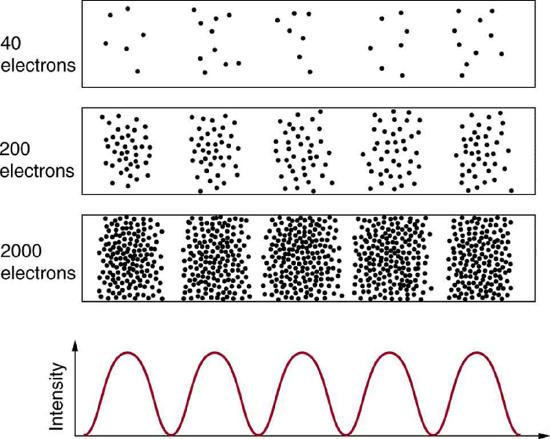
After de Broglie proposed the wave nature of matter, many physicists, including Schrödinger and Heisenberg, explored the consequences. The idea quickly emerged that, because of its wave character, a particle’s trajectory and destination cannot be precisely predicted for each particle individually. However, each particle goes to a definite place (Figure 1.9.1 ). After compiling enough data, you get a distribution related to the particle’s wavelength and diffraction pattern. There is a certain probability of finding the particle at a given location, and the overall pattern is called a probability distribution. Those who developed quantum mechanics devised equations that predicted the probability distribution in various circumstances.
It is somewhat disquieting to think that you cannot predict exactly where an individual particle will go, or even follow it to its destination. Let us explore what happens if we try to follow a particle. Consider the double-slit patterns obtained for electrons and photons in Figure 1.9.2 . The interferrence patterns build up statistically as individual particles fall on the detector. This can be observed for photons or electrons—for now, let us concentrate on electrons. You might imagine that the electrons are interfering with one another as any waves do. To test this, you can lower the intensity until there is never more than one electron between the slits and the screen. The same interference pattern builds up!
This implies that a particle’s probability distribution spans both slits, and the particles actually interfere with themselves. Does this also mean that the electron goes through both slits? An electron is a basic unit of matter that is not divisible. But it is a fair question, and so we should look to see if the electron traverses one slit or the other, or both. One possibility is to have coils around the slits that detect charges moving through them. What is observed is that an electron always goes through one slit or the other; it does not split to go through both.
But there is a catch. If you determine that the electron went through one of the slits, you no longer get a double slit pattern—instead, you get single slit interference. There is no escape by using another method of determining which slit the electron went through. Knowing the particle went through one slit forces a single-slit pattern. If you do not observe which slit the electron goes through, you obtain a double-slit pattern. How does knowing which slit the electron passed through change the pattern? The answer is fundamentally important—measurement affects the system being observed. Information can be lost, and in some cases it is impossible to measure two physical quantities simultaneously to exact precision. For example, you can measure the position of a moving electron by scattering light or other electrons from it. Those probes have momentum themselves, and by scattering from the electron, they change its momentum in a manner that loses information. There is a limit to absolute knowledge, even in principle.
Heisenberg’s Uncertainty Principle
It is mathematically possible to express the uncertainty that, Heisenberg concluded, always exists if one attempts to measure the momentum and position of particles. First, we must define the variable “x” as the position of the particle, and define “p” as the momentum of the particle. The momentum of a photon of light is known to simply be its frequency, expressed by the ratio \(h/λ\), where h represents Planck’s constant and \(\lambda\) represents the wavelength of the photon. The position of a photon of light is simply its wavelength (\(\lambda\)). To represent finite change in quantities, the Greek uppercase letter delta, or Δ, is placed in front of the quantity. Therefore,
\[\Delta{p}=\dfrac{h}{\lambda} \label{1.9.1} \]
\[\Delta{x}= \lambda \label{1.9.2} \]
By substituting \(\Delta{x}\) for \(\lambda\) into Equation \(\ref{1.9.1}\), we derive
\[\Delta{p}=\dfrac{h}{\Delta{x}} \label{1.9.3} \]
or,
\[\underset{\text{early form of uncertainty principle }}{\Delta{p}\Delta{x}=h} \label{1.9.4} \]
Equation \(\ref{1.9.4}\) can be derived by assuming the particle of interest is behaving as a particle, and not as a wave. Simply let \(\Delta p=mv\), and \(Δx=h/(m v)\) (from De Broglie’s expression for the wavelength of a particle). Substituting in \(Δp\) for \(mv\) in the second equation leads to Equation \(\ref{1.9.4}\).
Equation \ref{1.9.4} was further refined by Heisenberg and his colleague Niels Bohr, and was eventually rewritten as
\[\Delta{p_x}\Delta{x} \ge \dfrac{h}{4\pi} = \dfrac{\hbar}{2} \label{1.9.5} \]
with \(\hbar = \dfrac{h}{2\pi}= 1.0545718 \times 10^{-34}\; m^2 \cdot kg / s\).
Equation \(\ref{1.9.5}\) reveals that the more accurately a particle’s position is known (the smaller \(Δx\) is), the less accurately the momentum of the particle in the x direction (\(Δp_x\)) is known. Mathematically, this occurs because the smaller \(Δx\) becomes, the larger \(Δp_x\) must become in order to satisfy the inequality. However, the more accurately momentum is known the less accurately position is known (Figure 1.9.2 ).
Equation \(\ref{1.9.5}\) relates the uncertainty of momentum and position. An immediate questions that arise is if \(\Delta x\) represents the full range of possible \(x\) values or if it is half (e.g., \(\langle x \rangle \pm \Delta x\)). \(\Delta x\) is the standard deviation and is a statistic measure of the spread of \(x\) values. The use of half the possible range is more accurate estimate of \(\Delta x\). As we will demonstrated later, once we construct a wavefunction to describe the system, then both \(x\) and \(\Delta x\) can be explicitly derived. However for now, Equation \ref{1.9.5} will work.
For example: If a problem argues a particle is trapped in a box of length, \(L\), then the uncertainly of it position is \(\pm L/2\). So the value of \(\Delta x\) used in Equation \(\ref{1.9.5}\) should be \(L/2\), not \(L\).
An electron is confined to the size of a magnesium atom with a 150 pm radius. What is the minimum uncertainty in its velocity?
Solution
The uncertainty principle (Equation \(\ref{1.9.5}\)):
\[\Delta{p}\Delta{x} \ge \dfrac{\hbar}{2} \nonumber \]
can be written
\[\Delta{p} \ge \dfrac{\hbar}{2 \Delta{x}} \nonumber \]
and substituting \(\Delta p=m \Delta v \) since the mass is not uncertain.
\[\Delta{v} \ge \dfrac{\hbar}{2\; m\; \Delta{x}} \nonumber \]
the relevant parameters are
- mass of electron \(m=m_e= 9.109383 \times 10^{-31}\; kg\)
- uncertainty in position: \(\Delta x=150 \times 10^{-12} m \)
\[ \begin{align*} \Delta{v} &\ge \dfrac{1.0545718 \times 10^{-34} \cancel{kg} m^{\cancel{2}} / s}{(2)\;( 9.109383 \times 10^{-31} \; \cancel{kg}) \; (150 \times 10^{-12} \; \cancel{m}) } \\[4pt] &= 3.9 \times 10^5\; m/s \end{align*} \nonumber \]
What is the maximum uncertainty of velocity the electron described in Example 1.9.1 ?
- Answer
-
Infinity. There is no limit in the maximum uncertainty, just the minimum uncertainty.
Understanding the Uncertainty Principle through Wave Packets and the Slit Experiment
It is hard for most people to accept the uncertainty principle, because in classical physics the velocity and position of an object can be calculated with certainty and accuracy. However, in quantum mechanics, the wave-particle duality of electrons does not allow us to accurately calculate both the momentum and position because the wave is not in one exact location but is spread out over space. A "wave packet" can be used to demonstrate how either the momentum or position of a particle can be precisely calculated, but not both of them simultaneously. An accumulation of waves of varying wavelengths can be combined to create an average wavelength through an interference pattern: this average wavelength is called the "wave packet". The more waves that are combined in the "wave packet", the more precise the position of the particle becomes and the more uncertain the momentum becomes because more wavelengths of varying momenta are added. Conversely, if we want a more precise momentum, we would add less wavelengths to the "wave packet" and then the position would become more uncertain. Therefore, there is no way to find both the position and momentum of a particle simultaneously.
Several scientists have debated the Uncertainty Principle, including Einstein. Einstein created a slit experiment to try and disprove the Uncertainty Principle. He had light passing through a slit, which causes an uncertainty of momentum because the light behaves like a particle and a wave as it passes through the slit. Therefore, the momentum is unknown, but the initial position of the particle is known. Here is a video that demonstrates particles of light passing through a slit and as the slit becomes smaller, the final possible array of directions of the particles becomes wider. As the position of the particle becomes more precise when the slit is narrowed, the direction, or therefore the momentum, of the particle becomes less known as seen by a wider horizontal distribution of the light.
The speed of a 1.0 g projectile is known to within \(10^{-6}\;m/s\).
- Calculate the minimum uncertainty in its position.
- What is the maximum uncertainty of its position?
Solution
a
From Equation \(\ref{1.9.5}\), the \(\Delta{p_x} = m \Delta v_x\) with \(m=1.0\;g\). Solving for \(\Delta{x}\) to get
\[ \begin{align*} \Delta{x} &= \dfrac{\hbar}{2m\Delta v} \\[4pt] &= \dfrac{1.0545718 \times 10^{-34} \; m^2 \cdot kg / s}{(2)(0.001 \; kg)(10^{-6} \;m/s)} \\[4pt] &= 5.3 \times 10^{-26} \,m \end{align*} \nonumber \]
This negligible for all intents and purpose as expected for any macroscopic object.
b
Unlimited (or the size of the universe). The Heisenberg uncertainty principles does not quantify the maximum uncertainty.
Estimate the minimum uncertainty in the speed of an electron confined to a hydrogen atom within a diameter of \(1 \times 10^{-10} m\)?
- Answer
-
We need to quantify the uncertainty of the electron in position. We can estimate that as \(\pm 5 \times 10^{-10} m\). Hence, substituting the relavant numbers into Equation \ref{1.9.5} and solving for \(\Delta v\) we get
\[\Delta v= 1.15 \times 10^6\, km/s \nonumber \]
Notice that the uncertainty is significantly greater for the electron in a hydrogen atom than in the magnesium atom (Example 1.9.1 ) as expected since the magnesium atom is appreciably bigger.
Heisenberg’s Uncertainty Principle not only helped shape the new school of thought known today as quantum mechanics, but it also helped discredit older theories. Most importantly, the Heisenberg Uncertainty Principle made it obvious that there was a fundamental error in the Bohr model of the atom. Since the position and momentum of a particle cannot be known simultaneously, Bohr’s theory that the electron traveled in a circular path of a fixed radius orbiting the nucleus was obsolete. Furthermore, Heisenberg’s uncertainty principle, when combined with other revolutionary theories in quantum mechanics, helped shape wave mechanics and the current scientific understanding of the atom.
- Heisenberg get pulled over for speeding by the police. The officer asks him "Do you know how fast you were going?"
- Heisenberg replies, "No, but we know exactly where we are!"
- The officer looks at him confused and says "you were going 108 miles per hour!"
- Heisenberg throws his arms up and cries, "Great! Now we're lost!"