
3.9: Particle in a Finite Box and Tunneling (optional)
- Page ID
- 142970
\( \newcommand{\vecs}[1]{\overset { \scriptstyle \rightharpoonup} {\mathbf{#1}} } \)
\( \newcommand{\vecd}[1]{\overset{-\!-\!\rightharpoonup}{\vphantom{a}\smash {#1}}} \)
\( \newcommand{\dsum}{\displaystyle\sum\limits} \)
\( \newcommand{\dint}{\displaystyle\int\limits} \)
\( \newcommand{\dlim}{\displaystyle\lim\limits} \)
\( \newcommand{\id}{\mathrm{id}}\) \( \newcommand{\Span}{\mathrm{span}}\)
( \newcommand{\kernel}{\mathrm{null}\,}\) \( \newcommand{\range}{\mathrm{range}\,}\)
\( \newcommand{\RealPart}{\mathrm{Re}}\) \( \newcommand{\ImaginaryPart}{\mathrm{Im}}\)
\( \newcommand{\Argument}{\mathrm{Arg}}\) \( \newcommand{\norm}[1]{\| #1 \|}\)
\( \newcommand{\inner}[2]{\langle #1, #2 \rangle}\)
\( \newcommand{\Span}{\mathrm{span}}\)
\( \newcommand{\id}{\mathrm{id}}\)
\( \newcommand{\Span}{\mathrm{span}}\)
\( \newcommand{\kernel}{\mathrm{null}\,}\)
\( \newcommand{\range}{\mathrm{range}\,}\)
\( \newcommand{\RealPart}{\mathrm{Re}}\)
\( \newcommand{\ImaginaryPart}{\mathrm{Im}}\)
\( \newcommand{\Argument}{\mathrm{Arg}}\)
\( \newcommand{\norm}[1]{\| #1 \|}\)
\( \newcommand{\inner}[2]{\langle #1, #2 \rangle}\)
\( \newcommand{\Span}{\mathrm{span}}\) \( \newcommand{\AA}{\unicode[.8,0]{x212B}}\)
\( \newcommand{\vectorA}[1]{\vec{#1}} % arrow\)
\( \newcommand{\vectorAt}[1]{\vec{\text{#1}}} % arrow\)
\( \newcommand{\vectorB}[1]{\overset { \scriptstyle \rightharpoonup} {\mathbf{#1}} } \)
\( \newcommand{\vectorC}[1]{\textbf{#1}} \)
\( \newcommand{\vectorD}[1]{\overrightarrow{#1}} \)
\( \newcommand{\vectorDt}[1]{\overrightarrow{\text{#1}}} \)
\( \newcommand{\vectE}[1]{\overset{-\!-\!\rightharpoonup}{\vphantom{a}\smash{\mathbf {#1}}}} \)
\( \newcommand{\vecs}[1]{\overset { \scriptstyle \rightharpoonup} {\mathbf{#1}} } \)
\(\newcommand{\longvect}{\overrightarrow}\)
\( \newcommand{\vecd}[1]{\overset{-\!-\!\rightharpoonup}{\vphantom{a}\smash {#1}}} \)
\(\newcommand{\avec}{\mathbf a}\) \(\newcommand{\bvec}{\mathbf b}\) \(\newcommand{\cvec}{\mathbf c}\) \(\newcommand{\dvec}{\mathbf d}\) \(\newcommand{\dtil}{\widetilde{\mathbf d}}\) \(\newcommand{\evec}{\mathbf e}\) \(\newcommand{\fvec}{\mathbf f}\) \(\newcommand{\nvec}{\mathbf n}\) \(\newcommand{\pvec}{\mathbf p}\) \(\newcommand{\qvec}{\mathbf q}\) \(\newcommand{\svec}{\mathbf s}\) \(\newcommand{\tvec}{\mathbf t}\) \(\newcommand{\uvec}{\mathbf u}\) \(\newcommand{\vvec}{\mathbf v}\) \(\newcommand{\wvec}{\mathbf w}\) \(\newcommand{\xvec}{\mathbf x}\) \(\newcommand{\yvec}{\mathbf y}\) \(\newcommand{\zvec}{\mathbf z}\) \(\newcommand{\rvec}{\mathbf r}\) \(\newcommand{\mvec}{\mathbf m}\) \(\newcommand{\zerovec}{\mathbf 0}\) \(\newcommand{\onevec}{\mathbf 1}\) \(\newcommand{\real}{\mathbb R}\) \(\newcommand{\twovec}[2]{\left[\begin{array}{r}#1 \\ #2 \end{array}\right]}\) \(\newcommand{\ctwovec}[2]{\left[\begin{array}{c}#1 \\ #2 \end{array}\right]}\) \(\newcommand{\threevec}[3]{\left[\begin{array}{r}#1 \\ #2 \\ #3 \end{array}\right]}\) \(\newcommand{\cthreevec}[3]{\left[\begin{array}{c}#1 \\ #2 \\ #3 \end{array}\right]}\) \(\newcommand{\fourvec}[4]{\left[\begin{array}{r}#1 \\ #2 \\ #3 \\ #4 \end{array}\right]}\) \(\newcommand{\cfourvec}[4]{\left[\begin{array}{c}#1 \\ #2 \\ #3 \\ #4 \end{array}\right]}\) \(\newcommand{\fivevec}[5]{\left[\begin{array}{r}#1 \\ #2 \\ #3 \\ #4 \\ #5 \\ \end{array}\right]}\) \(\newcommand{\cfivevec}[5]{\left[\begin{array}{c}#1 \\ #2 \\ #3 \\ #4 \\ #5 \\ \end{array}\right]}\) \(\newcommand{\mattwo}[4]{\left[\begin{array}{rr}#1 \amp #2 \\ #3 \amp #4 \\ \end{array}\right]}\) \(\newcommand{\laspan}[1]{\text{Span}\{#1\}}\) \(\newcommand{\bcal}{\cal B}\) \(\newcommand{\ccal}{\cal C}\) \(\newcommand{\scal}{\cal S}\) \(\newcommand{\wcal}{\cal W}\) \(\newcommand{\ecal}{\cal E}\) \(\newcommand{\coords}[2]{\left\{#1\right\}_{#2}}\) \(\newcommand{\gray}[1]{\color{gray}{#1}}\) \(\newcommand{\lgray}[1]{\color{lightgray}{#1}}\) \(\newcommand{\rank}{\operatorname{rank}}\) \(\newcommand{\row}{\text{Row}}\) \(\newcommand{\col}{\text{Col}}\) \(\renewcommand{\row}{\text{Row}}\) \(\newcommand{\nul}{\text{Nul}}\) \(\newcommand{\var}{\text{Var}}\) \(\newcommand{\corr}{\text{corr}}\) \(\newcommand{\len}[1]{\left|#1\right|}\) \(\newcommand{\bbar}{\overline{\bvec}}\) \(\newcommand{\bhat}{\widehat{\bvec}}\) \(\newcommand{\bperp}{\bvec^\perp}\) \(\newcommand{\xhat}{\widehat{\xvec}}\) \(\newcommand{\vhat}{\widehat{\vvec}}\) \(\newcommand{\uhat}{\widehat{\uvec}}\) \(\newcommand{\what}{\widehat{\wvec}}\) \(\newcommand{\Sighat}{\widehat{\Sigma}}\) \(\newcommand{\lt}{<}\) \(\newcommand{\gt}{>}\) \(\newcommand{\amp}{&}\) \(\definecolor{fillinmathshade}{gray}{0.9}\)- Understand the basics of quantum tunneling and when to expect it be observable phenomenon
- Understand how the wavefunction and energies of the particle in a box changes when the box has finite heights (not infinite potential)
- Introduce the concept of binding energies
Tunneling Through a Barrier
Tunneling is a quantum mechanical phenomenon when a particle is able to penetrate through a potential energy barrier that is higher in energy than the particle’s kinetic energy. This amazing property of microscopic particles play important roles in explaining several physical phenomena including radioactive decay. Additionally, the principle of tunneling leads to the development of Scanning Tunneling Microscope (STM) which had a profound impact on chemical, biological and material science research.
Consider a ball rolling from one valley to another over a hill (Figure \(\PageIndex{1}\)). If the ball has enough energy (\(E\)) to overcome the potential energy (\(V\)) at the top of the barrier between each valley, then it can roll from one valley to the other. This is the classical picture and is controlled by the simple Law of Conservation of Energy approach taught in beginning physics courses. However, If the ball does not have enough kinetic energy (\(E<V\)), to overcome the barrier it will never roll from one valley to the other. In contrast, when quantum effects are taken into effect, the ball can "tunnel" through the barrier to the other valley, even if its kinetic energy is less than the potential energy of the barrier to the top of one of the hills.


The reason for the difference between classical and quantum motion comes from wave-particle nature of matter. One interpretation of this duality involves the Heisenberg uncertainty principle, which defines a limit on how precisely the position and the momentum of a particle can be known at the same time. This implies that there are no solutions with a probability of exactly zero (or one), though a solution may approach infinity if, for example, the calculation for its position was taken as a probability of 1, the other, i.e. its speed, would have to be infinity. Hence, the probability of a given particle's existence on the opposite side of an intervening barrier is non-zero, and such particles will appear on the 'other' (a semantically difficult word in this instance) side with a relative frequency proportional to this probability.
Microscopic particles such as protons, or electrons would behave differently as a consequence of wave-particle duality. Consider a particle with energy \(E\) that is confined in a box which has a barrier of height \(V\). Classically, the box will prevent these particles from escaping due to the insufficiency in kinetic energy of these particles to get over the barrier. However, if the thickness of the barrier is thin, the particles have some probability of penetrating through the barrier without sufficient energy and appear on the other side of the box (Figure \(\PageIndex{2}\)).
Tunneling is found from the Schrödinger equation, so we will start there. To simplify the calculations, the time-independent, one-dimensional Schrödinger equation is used (Equation \ref{eq1}).
\[ -{\frac{\hbar^2}{2m}} {\frac{\partial^2 \psi}{\partial x^2}} + V(r) \psi = E \psi \label{eq1}\]
To find solutions to a particular system, the potential \(V (x)\) must be defined. In this case, we will set the potential to zero for all space, except for the region between 0 and \(a\), which we will set as \(V_0\). This is represented by the piecewise function in Equation \ref{eq2}.
\[
V =
\begin{cases}
0 & \text{if } -\infty<x\leq 0\\[3pt]
V_0 & \text{if } 0<x<a\\[3pt]
0 & \text{if } a\leq x<\infty
\end{cases}
\label{eq2}\]
To solve this, the equation must be solved separately for each region. However, the boundary conditions at 0 and \(a\) for each region must be consistent such that \(\psi (x)\) is continuous for all \(x\), so that \(\psi (x)\) is a valid wavefunction. The general solution for each region, before applying the boundary conditions, is then
\[
\psi =
\begin{cases}
A\sin kx + B\cos kx & \text{if } -\infty<x\leq 0\\[3pt]
Ce^{-\alpha x} + De^{\alpha x} & \text{if } 0<x<a\\[3pt]
E\sin kx + F\cos kx & \text{if } a\leq x<\infty
\end{cases}
\]
where
\[k = \dfrac{\sqrt{2mE}}{\hbar} \]
and
\[\alpha = \dfrac{\sqrt{2m(V_o -E)}}{\hbar}.\]
To enforce continuity, the boundaries of each region are set equal. This is expressed as \(\psi_1 (0) = \psi_2 (0) \) and \(\psi_1 (a) = \psi_2 (a) \).
\[A\sin 0 + B\cos 0 = Ce^{0} + De^{0}\]
which implies that \( A=0 \), and \( B=C+D \). At the opposite boundary,
\[A\sin ka + B\cos ka = Ce^{-\alpha a} + De^{\alpha a}\]
It may be observed that, as \( a \) goes to infinity, the right hand side of this equation goes to infinity, which does not make physical sense. To reconcile this, \( D \) is set to zero. For the final region, \( E \) and \( F \), present a potentially intractable problem. However, if one realizes that the value at the boundary \( a \) is driving the wave in the region \( a \) to \( \infty \), it may also be realized that the wavefunction could be rewritten as \( Ce^{-\alpha a}\cos(k(x-a)) \), phase shifting the wavefunction by the value of \( a \) and setting the amplitude to the boundary value. The wavefunction is then
\[
\psi =
\begin{cases}
B\cos kx & \text{if } -\infty<x\leq 0\\[3pt]
Be^{-\alpha x} & \text{if } 0<x<a\\[3pt]
Be^{-\alpha a}\cos(k(x-a)) & \text{if } a\leq x<\infty
\end{cases}
\]
The amplitude of the wavefunction before the barrier is \(B\) and after the barrier is \(Be^{-\alpha a}\) where \( a \) represents the width of the barrier. So barrier attenuates the wavefunction by
\[ \exp \left [ -a \dfrac{\sqrt{2m(V_o -E)}}{\hbar} \right] \nonumber\]
where \( (V_o -E) \) is the difference between the potential energy of the barrier and the current energy of the particle (Figure \(\PageIndex{2}\)).
Since the square of the wavefunction is the probability distribution, the probability of transmission through a barrier is
\[P_t= \exp \left[-2a \dfrac{\sqrt{2m(V_o -E)}}{\hbar} \right] \label{trans}\]
As the barrier width or height approaches zero, the probability of a particle traveling through the barrier becomes 1. Also of note is that \( k \) is unchanged on the other side of the barrier. This implies that the energy of the particles are exactly the same as it was before they tunneled through the barrier, as stated earlier, the only thing that changes is the quantity of particles going in that direction. The rest are reflected off the barrier, and go back the way they came.
An electron having total kinetic energy \(E\) of 4.50 eV approaches a rectangular energy barrier with \(V= 5.00\, eV\) and \(L= 950\, pm\). Classically, the electron cannot pass through the barrier because \(E<V\). Calculate probability of tunneling of this electron through the barrier.
Solution
This is a straightforward application of Equation \ref{trans}. The electronvolt (eV) is a unit of energy that is equal to approximately \(1.6 \times 10^{−19}\; J\), which is the conversion used below.
The mass of an electron is \(9.10 \times 10^{-31}\; kg\)
\[\begin{align*} P &= \exp \left[\left( \dfrac{ (2) (950 \times 10^{-12}\, m) (\pi)}{ 1.0546 \times 10^{-34} m^2 kg / s} \right) \sqrt{(2)(9.10 \times 10^{-31}\; kg) (5.00 - 4.50 \; \cancel{eV})( 1.60 \times 10^{-19} J/\cancel{eV}) } \right] \\[4pt] &= \exp^{-6.88} = 1.03 \times 10^{-3} \end{align*}\]
There is a ~0.1% probability of the electrons tunneling though the barrier.
While tunneling is always possible for any system with finite height barriers, for a particle to appreciably tunnel through a barrier three conditions must be met.
- The height of the barrier must be finite and the thickness of the barrier should be thin.
- The potential energy of the barrier exceeds the kinetic energy of the particle (\(E<V\)).
- The particle has wave properties because the wavefunction is able to penetrate through the barrier. This suggests that quantum tunneling only apply to microscopic objects such protons or electrons and does not apply to macroscopic objects.
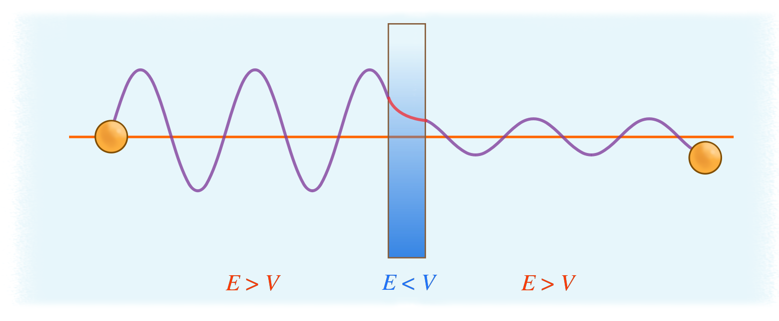
If these conditions are met, there would be some probability of finding the particles on the other side of the barrier. Beginning as a sinusoidal wave, a particle begins tunneling through the barrier and goes into exponential decay until it exits the barrier and gets transmitted out the other side as a final sinusoidal wave with a smaller amplitude. The act of tunneling decreases the wave amplitude due the reflection of the incident wave when it comes into the contact with the barrier but does not affect the wave equation.
Tunneling in a Particle in a Finite Height Box
The finite potential well is an extension of the infinite potential well from the previous section. The main difference between these two systems is that now the particle has a non-zero probability of finding itself outside the well, although its kinetic energy is less than that required, according to classical mechanics, for scaling the potential barrier. This type of problem is more realistic, but more difficult to solve due to the yielding of transcendental equations. The particle is again confined to a box, but one which has finite, not infinite, potential walls. We consider a potential well of height \(V_0\) (Figure \(\PageIndex{3}\)).

We have the following potential, \(V(x)\), given by the boundary conditions shown in Figure \(\PageIndex{3}\):
\[V(x)=\left\{\begin{array}{ll}
-V_{0} & |x|<L \\
0 & |x|>L
\end{array}\right.\]
In this example, the origin of the x-axis was chosen at the center of the well. By doing so, the potential is symmetric about \(x=0\), giving rise to parity (Note: this could also be applied to a symmetric infinite wells). For the finite well, two cases must be distinguished, corresponding to positive or negative values of the energy \(E\). It is possible for the particle to be bound, or unbound. The case \(E<0\) corresponds to a particle which is confined (and whose energy is less than the well depth) and hence is in a bound state [1]. When \(E>0\), the particle is unconfined and corresponds to a scattering problem. The latter case will only briefly be discussed.
Figure \(\PageIndex{4}\) provides a prelude to what the wavefunctions and probability distributions for several states will look like in a finite well. Comparing Figure \(\PageIndex{4}\) with the infinite case, we see that in the finite case, the wavefunctions do not have to be zero at the walls of the well. In the finite case, the wavelengths are slightly longer, implying that the allowed energies will be somewhat smaller.

Bound States
In the bound state we have,\(−V_0<=E<0\) (since \(E\) cannot be lower than the absolute minimum of the potential. The Schrödinger equation for the two regions is given by:
- \(|x|<L\) (inside the well): \[-\frac{\hbar^{2}}{2 m} \frac{\partial^{2}}{\partial x^{2}} \psi(x)-V_{0} \psi(x)=-|E| \psi(x)\]
- \(|x|>L\) (outside the well): \[-\frac{\hbar^{2}}{2 m} \frac{\partial^{2}}{\partial x^{2}} \psi(x)=-|E| \psi(x)\]
Here, the binding energy, \(|E|\) of the particle is introduced (\(|E|=-E\)). To simplify the Schrödinger equations, let,
\[\alpha=\sqrt{\frac{2 m}{\hbar^{2}}\left(V_{0}-|E|\right)}\]
and
\[\beta=\sqrt{\frac{2 m}{\hbar^{2}}|E|}\]
The solutions of the Schrödinger equation separate into even and odd functions, and we need only consider positive values of \(x\) (which could be inferred from the potential). With the application of the boundary conditions, the even solutions are given as
\[\psi^{F}(x)=\left\{\begin{array}{ll}
A \cos (\alpha \alpha) & 0<x<L \\
C e^{-\beta \hbar} & x>L
\end{array}\right.\]
and the odd solutions are given as
\[\psi^{o}(x)=\left\{\begin{array}{ll}
A \sin (\alpha \alpha) & 0<x<L \\
C e^{-\beta_{x}} & x>L
\end{array}\right.\]
Despite the discontinuous nature of the potential at \(x=L\), the wavefunction and its derivative are still continuous, and these conditions provide the required boundary conditions to determine the quantized energies. The requirements that \(ψ_O=\psi E(x)\) and yields two equations:
\[\begin{array}{l}
A \cos (\alpha L)=C e^{-\beta L} \\
-\alpha A \sin (\alpha L)=-\beta C e^{-\beta L}
\end{array}\]
These can be combined to give the even eigenvalue condition (which depends on the energies but not on the constants \(A\) and \(C\)) is
\[\alpha \tan (\alpha L)=\beta\]
The odd eigenvalue condition is found to be
\[\alpha \cot (\alpha L)=-\beta\]
The energy levels of the bound states are found by solving these transcendental equations, either graphically or numerically. In doing so, it is helpful to change to dimensionless variables. We introduce the dimensionless quantities
\[\begin{array}{l}
\xi=\alpha L \\
\eta=\beta L
\end{array}\]
Upon substitution these quantities, the transcendental equations become
- Even States: \(\xi \tan \xi=\eta\)
- Odd States: \(\xi \cot \xi=-\eta\)
The graphical determination of the energy levels are obtained by finding the points of intersection of the circle (Figure \(\PageIndex{3}\))
\[\xi^{2}+\eta^{2}=\gamma^{2}\]
where γ is of known radius (found by simple substitution),
\[\gamma=\sqrt{\frac{2 m V_{o} L^{2}}{\hbar^{2}}}\]

What can be concluded from Figure \(\PageIndex{5}\)?
- The bound-state energy levels are non-degenerate.
- The bound-state energy levels are finite, but increase without bound and depend on the parameter \(γ\). Thus, deeper and wider potentials have a larger number of bound states.
- The bound state spectrum consists of alternating even and odd states, with the ground state always being even.
Unbound States
The finite well problem shows that wavefunctions are not localized in the vicinity of the well. This is the case of unbound states, where eigenvalues of energy are a continuum. In this problem, a particle is incident upon the well from the left, interacts with the well, and gets transmitted or reflected. The solution of the Schrödinger equation is outlined briefly. Note that in one dimension, there is a lack of symmetry between the external regions to the left and right of the potential, since the particle is assumed to be incident on the potential in a given direction. Therefore, there is no need to exercise parity.
For the external regions, the solution of the Schrödinger equation is given by
\[\psi(x)=\left\{\begin{array}{ll}
A e^{\mid \alpha_{\alpha}}+B e^{-i b} & x<-L \\
C e^{\mid \alpha,} & x>L
\end{array}\right.\]
where
\[k=\sqrt{\frac{2 m E}{\hbar^{2}}}\]
In the region of x<−L, the wavefunction is seen to consist of an incident wave of amplitude \(A\) and \(a\) reflected wave of amplitude B. In the region of x>L, the wavefunction is seen as a pure transmitted wave of amplitude \(C\).
For the internal region, the solution of the Schrödinger equation is given by
\[\psi(x)=F e^{i \omega}+G e^{-i \omega}\]
where
\[\alpha=\sqrt{\frac{2 m}{\hbar^{2}}\left(V_{0}+E\right)}\]
By applying continuity at \(x=L\) and \(x=−L\), \(F\) and \(G\) are eliminated and the ratios of B/A and C/A can be solved to obtain the reflection coefficient, R=|B/A|2, and the transmission coefficient, T=|C/A|2. An important aspect to briefly point out is that the transmission coefficient is generally less than unity, which is in contradiction to the classical prediction that suggests that the particle should always be transmitted
Summary
Quantum tunneling is a phenomenon where particles may "tunnel through" a barrier which they have insufficient kinetic energy to overcome according to classical mechanics. Tunneling is a result of the wavelike nature of quantum particles, and cannot be predicted by any classical system. The major differences between a particle in a finite box and an infinite well are:
- Only a finite number of energy levels exist (bound state)
- Tunneling into the barrier (wall) is possible
- Higher energy states are less tightly bound than lower ones
- A particle provided with enough energy can escape the well (unbound state)