
Lab 8: Quantifying Protein Concentration
- Page ID
- 2381
\( \newcommand{\vecs}[1]{\overset { \scriptstyle \rightharpoonup} {\mathbf{#1}} } \)
\( \newcommand{\vecd}[1]{\overset{-\!-\!\rightharpoonup}{\vphantom{a}\smash {#1}}} \)
\( \newcommand{\id}{\mathrm{id}}\) \( \newcommand{\Span}{\mathrm{span}}\)
( \newcommand{\kernel}{\mathrm{null}\,}\) \( \newcommand{\range}{\mathrm{range}\,}\)
\( \newcommand{\RealPart}{\mathrm{Re}}\) \( \newcommand{\ImaginaryPart}{\mathrm{Im}}\)
\( \newcommand{\Argument}{\mathrm{Arg}}\) \( \newcommand{\norm}[1]{\| #1 \|}\)
\( \newcommand{\inner}[2]{\langle #1, #2 \rangle}\)
\( \newcommand{\Span}{\mathrm{span}}\)
\( \newcommand{\id}{\mathrm{id}}\)
\( \newcommand{\Span}{\mathrm{span}}\)
\( \newcommand{\kernel}{\mathrm{null}\,}\)
\( \newcommand{\range}{\mathrm{range}\,}\)
\( \newcommand{\RealPart}{\mathrm{Re}}\)
\( \newcommand{\ImaginaryPart}{\mathrm{Im}}\)
\( \newcommand{\Argument}{\mathrm{Arg}}\)
\( \newcommand{\norm}[1]{\| #1 \|}\)
\( \newcommand{\inner}[2]{\langle #1, #2 \rangle}\)
\( \newcommand{\Span}{\mathrm{span}}\) \( \newcommand{\AA}{\unicode[.8,0]{x212B}}\)
\( \newcommand{\vectorA}[1]{\vec{#1}} % arrow\)
\( \newcommand{\vectorAt}[1]{\vec{\text{#1}}} % arrow\)
\( \newcommand{\vectorB}[1]{\overset { \scriptstyle \rightharpoonup} {\mathbf{#1}} } \)
\( \newcommand{\vectorC}[1]{\textbf{#1}} \)
\( \newcommand{\vectorD}[1]{\overrightarrow{#1}} \)
\( \newcommand{\vectorDt}[1]{\overrightarrow{\text{#1}}} \)
\( \newcommand{\vectE}[1]{\overset{-\!-\!\rightharpoonup}{\vphantom{a}\smash{\mathbf {#1}}}} \)
\( \newcommand{\vecs}[1]{\overset { \scriptstyle \rightharpoonup} {\mathbf{#1}} } \)
\( \newcommand{\vecd}[1]{\overset{-\!-\!\rightharpoonup}{\vphantom{a}\smash {#1}}} \)
\(\newcommand{\avec}{\mathbf a}\) \(\newcommand{\bvec}{\mathbf b}\) \(\newcommand{\cvec}{\mathbf c}\) \(\newcommand{\dvec}{\mathbf d}\) \(\newcommand{\dtil}{\widetilde{\mathbf d}}\) \(\newcommand{\evec}{\mathbf e}\) \(\newcommand{\fvec}{\mathbf f}\) \(\newcommand{\nvec}{\mathbf n}\) \(\newcommand{\pvec}{\mathbf p}\) \(\newcommand{\qvec}{\mathbf q}\) \(\newcommand{\svec}{\mathbf s}\) \(\newcommand{\tvec}{\mathbf t}\) \(\newcommand{\uvec}{\mathbf u}\) \(\newcommand{\vvec}{\mathbf v}\) \(\newcommand{\wvec}{\mathbf w}\) \(\newcommand{\xvec}{\mathbf x}\) \(\newcommand{\yvec}{\mathbf y}\) \(\newcommand{\zvec}{\mathbf z}\) \(\newcommand{\rvec}{\mathbf r}\) \(\newcommand{\mvec}{\mathbf m}\) \(\newcommand{\zerovec}{\mathbf 0}\) \(\newcommand{\onevec}{\mathbf 1}\) \(\newcommand{\real}{\mathbb R}\) \(\newcommand{\twovec}[2]{\left[\begin{array}{r}#1 \\ #2 \end{array}\right]}\) \(\newcommand{\ctwovec}[2]{\left[\begin{array}{c}#1 \\ #2 \end{array}\right]}\) \(\newcommand{\threevec}[3]{\left[\begin{array}{r}#1 \\ #2 \\ #3 \end{array}\right]}\) \(\newcommand{\cthreevec}[3]{\left[\begin{array}{c}#1 \\ #2 \\ #3 \end{array}\right]}\) \(\newcommand{\fourvec}[4]{\left[\begin{array}{r}#1 \\ #2 \\ #3 \\ #4 \end{array}\right]}\) \(\newcommand{\cfourvec}[4]{\left[\begin{array}{c}#1 \\ #2 \\ #3 \\ #4 \end{array}\right]}\) \(\newcommand{\fivevec}[5]{\left[\begin{array}{r}#1 \\ #2 \\ #3 \\ #4 \\ #5 \\ \end{array}\right]}\) \(\newcommand{\cfivevec}[5]{\left[\begin{array}{c}#1 \\ #2 \\ #3 \\ #4 \\ #5 \\ \end{array}\right]}\) \(\newcommand{\mattwo}[4]{\left[\begin{array}{rr}#1 \amp #2 \\ #3 \amp #4 \\ \end{array}\right]}\) \(\newcommand{\laspan}[1]{\text{Span}\{#1\}}\) \(\newcommand{\bcal}{\cal B}\) \(\newcommand{\ccal}{\cal C}\) \(\newcommand{\scal}{\cal S}\) \(\newcommand{\wcal}{\cal W}\) \(\newcommand{\ecal}{\cal E}\) \(\newcommand{\coords}[2]{\left\{#1\right\}_{#2}}\) \(\newcommand{\gray}[1]{\color{gray}{#1}}\) \(\newcommand{\lgray}[1]{\color{lightgray}{#1}}\) \(\newcommand{\rank}{\operatorname{rank}}\) \(\newcommand{\row}{\text{Row}}\) \(\newcommand{\col}{\text{Col}}\) \(\renewcommand{\row}{\text{Row}}\) \(\newcommand{\nul}{\text{Nul}}\) \(\newcommand{\var}{\text{Var}}\) \(\newcommand{\corr}{\text{corr}}\) \(\newcommand{\len}[1]{\left|#1\right|}\) \(\newcommand{\bbar}{\overline{\bvec}}\) \(\newcommand{\bhat}{\widehat{\bvec}}\) \(\newcommand{\bperp}{\bvec^\perp}\) \(\newcommand{\xhat}{\widehat{\xvec}}\) \(\newcommand{\vhat}{\widehat{\vvec}}\) \(\newcommand{\uhat}{\widehat{\uvec}}\) \(\newcommand{\what}{\widehat{\wvec}}\) \(\newcommand{\Sighat}{\widehat{\Sigma}}\) \(\newcommand{\lt}{<}\) \(\newcommand{\gt}{>}\) \(\newcommand{\amp}{&}\) \(\definecolor{fillinmathshade}{gray}{0.9}\)Molecular absorption in the ultraviolet and visible region depends on the electronic structure of the absorbing molecule. Light energy is absorbed in quanta, elevating electrons from filled orbitals in the ground state to empty orbitals. Excited molecules return to the ground state, most often by radiationless transition, the absorbed energy appears in the system as heat. Since the frequency (or wavelength) of light absorbed is characteristic of the energy levels in a molecule, the UV-visible spectrum is often used as a method of qualitative analysis. However, quantitative analysis can also be performed using this technique as is demonstrated in this experiment.
Introduction
According to Beer's law, the decrease in light intensity observed when monochromatic light passes through an absorbing medium is related to the concentration of the absorbing species by the equation
\[\log \dfrac{I_o}{I} = A = \epsilon bc \label{1}\]
where \(I_o\) is the incident light intensity, \(I\), the emerging light intensity, \(A\), the absorbance, \(\epsilon\) is the molar absorptivity, \(b\), the path length in cm, and \(c\), the concentration of the absorbing species in moles/L. The transmittance T is defined to be the ratio I / Io so that
\[- \log T = A \label{2}\]
(Note that log refers to logarithms to the base 10). The molar absorptivity, \(\epsilon\), is not only characteristic of the absorbing molecule so that it depends on the wavelength of the incident light, but it also depends on the medium in which this molecule is dissolved, that is, on the nature of the solvent. Having established the value of \(\epsilon\) at a given wavelength for a given medium, an unknown concentration of the absorbing molecule can be determined by measuring A in a cell of fixed geometry.
A typical UV-visible spectrophotometer consists of a tungsten or deuterium lamp as sources of visible or UV radiation, respectively, a monochromator, a detector, normally, a photomultiplier tube, and amplifying and readout electronics. In a double beam instrument, the intensity transmitted through the solution of interest is compared with that passing through an identical cell containing only the solvent. In this way compensation is made for loss in intensity due to absorption by the solvent and glass, and for loss by reflectance. You will use a single beam instrument. The compensation is made for loss in intensity due to absorption by the solvent and glass, and for loss by reflectance. by collecting a spectrum of the cell containing only the solvent. Storing this spectrum in memory and then subtracting the “blank” spectrum from the spectrum of the solvent plus sample. Then \(I_o\) in Equation \(\ref{1}\) refers to the intensity after passing through the cell containing the solvent.
Just as you used visible spectroscopy to identify and quantify metal ions in solution in general chemistry lab, you can use UV-visible spectroscopy to measure protein concentrations in solution. Proteins are extremely important molecules in biochemistry. They make up a large portion of the human body, playing both a structural role and as important catalysts for biochemical reactions. Understanding protein function is a key to understanding life itself and the molecular basis of disease. Proteins are large polymers of many of the 20 amino acids. Figure 1 shows the chemical structure of each of the 20 amino acids. The pKa for the ionizable side chains are also given in the figure.

Figure 1: A guide to the twenty common Amino Acids. (CC BY-SA-NC, Compoundschem.com).
The side chains are connected by amide linkages between the amino acids. There is a free amino and free carboxylic acid group at each end. Figure 2 Several methods are used to measure protein concentrations. Some methods are direct and others are indirect. One can measure the UV absorbance of the solution at 250-300 nm, a direct method. The indirect assay, usually called a colorimetric assay, takes advantage of a color change of a compound upon binding to the protein.
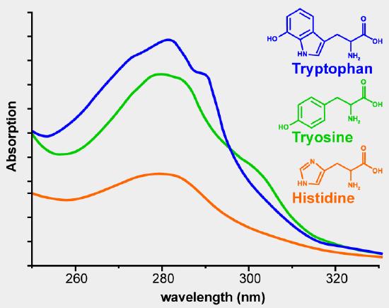
Using the absorbance at 280 nm is the simplest method. The aromatic side chains phenylalanine, tyrosine and tryptophan absorb UV radiation in the range of 250-300 nm. Figure 2 shows the UV absorbance spectra of phenylalanine, tyrosine and tryptophan. The extinction coefficient of a pure protein can be calculated from the number of tyrosine and tryptophan residues in the amino acid sequence. The extinction coefficients at 280 nm for the isolated amino acid side chains are 1200 M-1 cm-1 for tyrosine and 5600 M-1 cm–1 for tryptophan. If you know the sequence of the protein of interest and know that it is pure, you can use the absorbance at 280 nm to determine the concentration of your protein. If you have a mixture of proteins and want to know the total concentration of protein in the solution, in milk for example, this method would not work because you cannot calculate the extinction coefficient for a mixture of proteins. You can get a relative measure of the amount of protein present in solutions. The solution with the highest absorbance at 280 nm had the greatest protein concentration. This is a rash generalization because a dilute solution of a protein that contains many aromatic residues will have a greater absorbance than a more concentrated solution of a protein with few aromatic amino acids.
Colorimetric assays for protein have been developed to get around this problem. These assays use a compound that changes color in the presence of protein.
\[\text{Yellow compound} + \text{protein} \rightarrow \text{purple-protein complex}\]
The amount of purple color produced is proportional to the amount of protein present. The protein concentration of an unknown is determined by comparing the color produced by the “unknown” solution with the color produced by solutions of known protein, the standard curve.
There are many different compounds that are used. Two of the most important properties for the compound are: 1) that they interact with all proteins similarly and 2) that the absorbance spectrum of the unbound compound does not significantly overlap with the spectrum of the complex. The reagent coomassie brilliant blue is a blue dye that binds tightly to most proteins. There are 3 forms of coomassie blue that are in equilibrium with each other at low pH. In very acidic solutions the red form, positively charged of the dye is most stable above pH=2 the blue form, negatively charged blue form is more stable. Figure 3 shows the structure of the red and blue forms of coomassie brilliant blue. The intermediate neutral form is stable over a very narrow pH range and is difficult to stabilize, except in the presence of detergents.
By looking at the pKas for the amino acid side chains, you can see that at pH < 4 all proteins carry a net positive charge. The negatively charged blue form of the coomassie blue interacts with the proteins and is stabilized. The dye will bind to the protein until all of the positive charges are neutralized or all the dye is bound to the proteins. If the dye is in great excess (there is much more dye than protein in solution), then the amount of blue color produced is proportional to the protein concentration in solution. If the amount of dye is not much greater than the amount of protein, the dye will all be bound and the amount of color produced will no longer be a measure of the protein concentration. The dye solution becomes saturated.
To run a colorimemtric protein assay with any color producing compound, you must first create a standard curve. Due to differences in the reagent solution from batch to batch you must create a new standard curve every time you run the experiment. To make a standard curve, you make a series of solutions of known protein concentration. You may have to repeat the process until you find a range of concentrations for which the absorbance increases linearly, or almost linearly with protein concentration. If the amount of protein in solution is close to the dye concentration you will not get a linear relationship between concentration and absorbance. Once you have made your standard curve you can then compare the absorbance of your unknown to the standard curve and thereby determine the amount of protein in solution. It may be necessary to dilute your unknown to get an absorbance that is within the linear range of your standard curve. If you do this you must keep track of how much you dilute the sample and then use the dilution factor to calculate the final concentration of your undiluted sample.
The caveats for this type of assay are that the compounds may interact with different proteins to a different extent. The absorbance of a 1mg/ml solution of BSA, bovine serum albumin, might give a different reading than a 1mg/ml solution of collagen, a common structural protein.
In this laboratory exercise you will measure the concentration of a BSA solution by both methods. Keep in mind that the two methods are completely unrelated and there is no reason to expect the same absorbance readings for both assays on the same sample.
Experiment
Record absorbance spectra of the red and blue forms of coomassie blue. Do this on Day one of the experiment The red form at low pH: Prepare 10ml of a 0.02mM solution of coomassie blue by diluting the appropriate amount of the stock solution provided (concentration is given on the bottle) with 2.5M HCl. What volume of 0.1mM coomassie blue would you use? What is the pH of the resulting solution? The Blue form at pH 7: Prepare 10ml of a 0.02mM dye solution by diluting the appropriate volume of the stock solution with pH 7 buffer.
- Record the absorbance spectrum of the blue form of the dye from 390 to 800 nm.
- Record the absorbance at the wavelength of maximum absorbance (\(\lambda_{max}\))
- Then record the spectrum of the red dye over the same wavelength range.
- Record \(\lambda_{max}\) of the red form and the absorbance of the red form at the \(\lambda_{max}\) of the blue form.
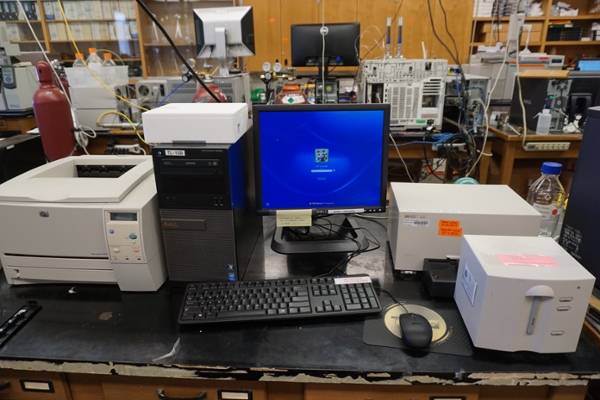
Simple Instructions for Operation of HP-8452A
The Agilent (HP) 8453 UV-Vis unit in room 3480 is pictured below.
- Turn on instrument using the power button. Wait 5 minutes for the instrument to warm up. When the indicator on the front turns green, launch the software.
- *** edit march 2018. Instructions from this point on are out of date, ask TA for advice!!! ***
- Click function key, top of keyboard, F4: Acquisition, set wavelength range to 390-800
- Put blank solution C into cuvette and put cuvette in sample holder. Make sure the clear sides face the instrument. Make sure you depress the lever on the side of the cell holder.
- Click function key F2 to measure the blank. This takes a spectrum of the solvent and cuvette and stores it in memory. This is then subtracted from all subsequent scans.
- Place the cuvette containing the sample in the cell holder. If you are using the same cuvette repeatedly, rinse the cuvette with the new solution before taking the spectrum.
- Click F1 (Measure sample). The spectrum will appear on the screen.
- Click F2 (Cursor control). Use the left and right arrows to find \(\lambda_{max}\) and any shoulders in your spectrum.
- Click F1 (Mark) at each wavelength you want to record with cursor position.
- Click F10 to return to the main menu.
- Click F9 (hardcopy) will print your spectrum with cursor marks and wavelengths indicated.
Measuring protein concentration
To determine the concentration of a protein solution you must first prepare a series of protein solutions of known concentration and construct a standard absorbance curve. Using the 2.00mg/ml stock solution prepare 10 ml of each of the following solutions. Use deionized water to make the solutions to volume. Day one, make the standard solutions. They are stable. You will do the assay on day 2 of the experiment.
Before coming to class calculate the volume of the 2.0 mg/ml stock solution you need for each solution. And complete this table:
| Volume of stock solution to add (mL) | Concentration | |
|---|---|---|
| Solution 1 | 0.1 mg/mL | |
| Solution2 | 0.2 mg/mL | |
| Solution3 | 0.4 mg/mL | |
| Solution4 | 0.6 mg/mL | |
| Solution5 | 0.8 mg/mL | |
| Solution6 | 1.0 mg/mL |
Volume of stock solution to add concentration Solution 1 0.1 mg/ml Solution 2 0.2 mg/ml Solution 3 0.4 mg/ml Solution 4 0.6 mg/ml Solution 5 0.8 mg/ml Solution 6 1.0 mg/ml Protein Assay: This will be done on day two of the experiment. Using the table below as a guide prepare the protein assay. Label 1 test tube “blank” Label 2 sets of 8 test tubes 1-8 Using the 5 ml pipette in your drawer pipette 5 ml of the protein assay reagent into the 17 test tubes. Use the automatic pipettor to add the protein solution (or the water) to the tube and vortex to mix thoroughly after adding the protein. Wait 10 minutes and then read the absorbance of each solution at 596 nm. Get 17 cuvettes from the stockroom. blank 100 ul water 1 100 ul 0.1mg/ml 2 100 ul 0.2mg/ml 3 100 ul 0.4mg/ml 4 100 ul 0.6mg/ml 5 100 ul 0.8mg/ml 6 100 ul 1.0mg/ml 7 100 ul 2.0 mg/ml 8 100 ul unknown Remember you will do all measurements(except the blank) in duplicate.
Now you will measure the absorbance at 596nm of standards and unknown
- Press F10 (return) will get you back to the acquisition window.
- Click F3 (functions) and use the down arrow to highlight “Fn 1:” and press ENTER. Select L1. When prompted enter the wavelength 596. Press ESC to return to the menu.
- Click F5 (options) and use the down arrow to highlight “wavelength list mode” and press ENTER.
- Now place your reagent blank in the sample holder and press F2 to measure the blank. Next measure the absorbance of solutions 1-8. You will see a list of absorbance measurements at the selected wavelength on the screen.
- Press F9 hardcopy to get a printout of the data. Make sure it prints before quitting the program.
UV spectrum of the unknown: Do this on day two of the experiment
Collect a UV spectrum of the unknown protein solution from 240nm to 340 nm. Use water as the blank. The molar absorptivity for bovine serum albumin (BSA) at 280 nm is 43,600 M-1cm-1. The molecular weight of BSA is 66,300 g/mol. Determine the absorbance at 280 nm calculate the concentration and compare it to that which you measure by the dye binding assay.
Analysis of the Data
- Calculate the molar absorptivities for the red and blue forms of coomassie blue each at their \(\lambda_{max}\).
- Calculate the molar absorptivity for the red form at the \(\lambda_{max}\) of the blue form.
- Make a table of the protein concentration and absorbance at 596 nm. Include both readings. Also plot the average value for each standard. It should be linear and should go through the origin. Use the standard curve to determine the concentration of protein in your unknown. If you are using excel or any other graphing/analysis package you must plot the standard curve as a full page and use a ruler to determine the protein concentration. If the absorbance of your unknown falls in the linear range of the standard curve, calculate an molar absorptivity for the BSA-coomassie complex using excel to calculate the best-fit line. Use this to determine the concentration of your unknown. If your graph is not linear, use the standard curve to determine the concentration graphically.
- Calculate the concentration of the unknown using the absorbance at 280nm. How well does it agree with the concentration found at 596 nm? Which do you consider to be more accurate, and why?
- Your report should include the spectra of the red and blue forms of coomassie blue, the UV spectrum of your unknown protein solution. All spectra should be annotated with the required maximum absorbance. All the absorbance data from the standard curve and unknown.