
Appendix 3: Instrumental Instructions
- Page ID
- 432999
\( \newcommand{\vecs}[1]{\overset { \scriptstyle \rightharpoonup} {\mathbf{#1}} } \)
\( \newcommand{\vecd}[1]{\overset{-\!-\!\rightharpoonup}{\vphantom{a}\smash {#1}}} \)
\( \newcommand{\dsum}{\displaystyle\sum\limits} \)
\( \newcommand{\dint}{\displaystyle\int\limits} \)
\( \newcommand{\dlim}{\displaystyle\lim\limits} \)
\( \newcommand{\id}{\mathrm{id}}\) \( \newcommand{\Span}{\mathrm{span}}\)
( \newcommand{\kernel}{\mathrm{null}\,}\) \( \newcommand{\range}{\mathrm{range}\,}\)
\( \newcommand{\RealPart}{\mathrm{Re}}\) \( \newcommand{\ImaginaryPart}{\mathrm{Im}}\)
\( \newcommand{\Argument}{\mathrm{Arg}}\) \( \newcommand{\norm}[1]{\| #1 \|}\)
\( \newcommand{\inner}[2]{\langle #1, #2 \rangle}\)
\( \newcommand{\Span}{\mathrm{span}}\)
\( \newcommand{\id}{\mathrm{id}}\)
\( \newcommand{\Span}{\mathrm{span}}\)
\( \newcommand{\kernel}{\mathrm{null}\,}\)
\( \newcommand{\range}{\mathrm{range}\,}\)
\( \newcommand{\RealPart}{\mathrm{Re}}\)
\( \newcommand{\ImaginaryPart}{\mathrm{Im}}\)
\( \newcommand{\Argument}{\mathrm{Arg}}\)
\( \newcommand{\norm}[1]{\| #1 \|}\)
\( \newcommand{\inner}[2]{\langle #1, #2 \rangle}\)
\( \newcommand{\Span}{\mathrm{span}}\) \( \newcommand{\AA}{\unicode[.8,0]{x212B}}\)
\( \newcommand{\vectorA}[1]{\vec{#1}} % arrow\)
\( \newcommand{\vectorAt}[1]{\vec{\text{#1}}} % arrow\)
\( \newcommand{\vectorB}[1]{\overset { \scriptstyle \rightharpoonup} {\mathbf{#1}} } \)
\( \newcommand{\vectorC}[1]{\textbf{#1}} \)
\( \newcommand{\vectorD}[1]{\overrightarrow{#1}} \)
\( \newcommand{\vectorDt}[1]{\overrightarrow{\text{#1}}} \)
\( \newcommand{\vectE}[1]{\overset{-\!-\!\rightharpoonup}{\vphantom{a}\smash{\mathbf {#1}}}} \)
\( \newcommand{\vecs}[1]{\overset { \scriptstyle \rightharpoonup} {\mathbf{#1}} } \)
\(\newcommand{\longvect}{\overrightarrow}\)
\( \newcommand{\vecd}[1]{\overset{-\!-\!\rightharpoonup}{\vphantom{a}\smash {#1}}} \)
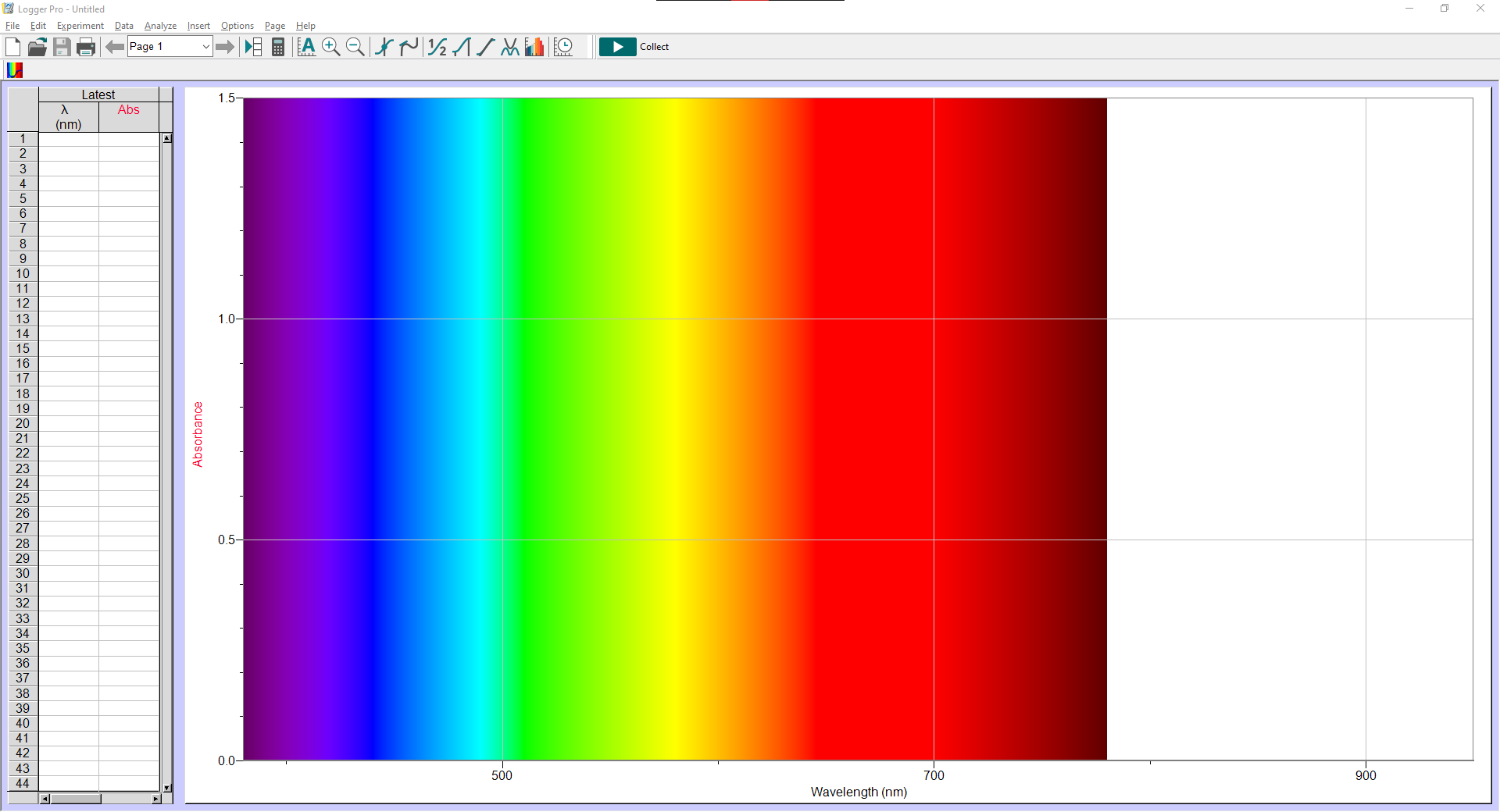
\(\newcommand{\avec}{\mathbf a}\) \(\newcommand{\bvec}{\mathbf b}\) \(\newcommand{\cvec}{\mathbf c}\) \(\newcommand{\dvec}{\mathbf d}\) \(\newcommand{\dtil}{\widetilde{\mathbf d}}\) \(\newcommand{\evec}{\mathbf e}\) \(\newcommand{\fvec}{\mathbf f}\) \(\newcommand{\nvec}{\mathbf n}\) \(\newcommand{\pvec}{\mathbf p}\) \(\newcommand{\qvec}{\mathbf q}\) \(\newcommand{\svec}{\mathbf s}\) \(\newcommand{\tvec}{\mathbf t}\) \(\newcommand{\uvec}{\mathbf u}\) \(\newcommand{\vvec}{\mathbf v}\) \(\newcommand{\wvec}{\mathbf w}\) \(\newcommand{\xvec}{\mathbf x}\) \(\newcommand{\yvec}{\mathbf y}\) \(\newcommand{\zvec}{\mathbf z}\) \(\newcommand{\rvec}{\mathbf r}\) \(\newcommand{\mvec}{\mathbf m}\) \(\newcommand{\zerovec}{\mathbf 0}\) \(\newcommand{\onevec}{\mathbf 1}\) \(\newcommand{\real}{\mathbb R}\) \(\newcommand{\twovec}[2]{\left[\begin{array}{r}#1 \\ #2 \end{array}\right]}\) \(\newcommand{\ctwovec}[2]{\left[\begin{array}{c}#1 \\ #2 \end{array}\right]}\) \(\newcommand{\threevec}[3]{\left[\begin{array}{r}#1 \\ #2 \\ #3 \end{array}\right]}\) \(\newcommand{\cthreevec}[3]{\left[\begin{array}{c}#1 \\ #2 \\ #3 \end{array}\right]}\) \(\newcommand{\fourvec}[4]{\left[\begin{array}{r}#1 \\ #2 \\ #3 \\ #4 \end{array}\right]}\) \(\newcommand{\cfourvec}[4]{\left[\begin{array}{c}#1 \\ #2 \\ #3 \\ #4 \end{array}\right]}\) \(\newcommand{\fivevec}[5]{\left[\begin{array}{r}#1 \\ #2 \\ #3 \\ #4 \\ #5 \\ \end{array}\right]}\) \(\newcommand{\cfivevec}[5]{\left[\begin{array}{c}#1 \\ #2 \\ #3 \\ #4 \\ #5 \\ \end{array}\right]}\) \(\newcommand{\mattwo}[4]{\left[\begin{array}{rr}#1 \amp #2 \\ #3 \amp #4 \\ \end{array}\right]}\) \(\newcommand{\laspan}[1]{\text{Span}\{#1\}}\) \(\newcommand{\bcal}{\cal B}\) \(\newcommand{\ccal}{\cal C}\) \(\newcommand{\scal}{\cal S}\) \(\newcommand{\wcal}{\cal W}\) \(\newcommand{\ecal}{\cal E}\) \(\newcommand{\coords}[2]{\left\{#1\right\}_{#2}}\) \(\newcommand{\gray}[1]{\color{gray}{#1}}\) \(\newcommand{\lgray}[1]{\color{lightgray}{#1}}\) \(\newcommand{\rank}{\operatorname{rank}}\) \(\newcommand{\row}{\text{Row}}\) \(\newcommand{\col}{\text{Col}}\) \(\renewcommand{\row}{\text{Row}}\) \(\newcommand{\nul}{\text{Nul}}\) \(\newcommand{\var}{\text{Var}}\) \(\newcommand{\corr}{\text{corr}}\) \(\newcommand{\len}[1]{\left|#1\right|}\) \(\newcommand{\bbar}{\overline{\bvec}}\) \(\newcommand{\bhat}{\widehat{\bvec}}\) \(\newcommand{\bperp}{\bvec^\perp}\) \(\newcommand{\xhat}{\widehat{\xvec}}\) \(\newcommand{\vhat}{\widehat{\vvec}}\) \(\newcommand{\uhat}{\widehat{\uvec}}\) \(\newcommand{\what}{\widehat{\wvec}}\) \(\newcommand{\Sighat}{\widehat{\Sigma}}\) \(\newcommand{\lt}{<}\) \(\newcommand{\gt}{>}\) \(\newcommand{\amp}{&}\) \(\definecolor{fillinmathshade}{gray}{0.9}\)Logger Pro with Spectrophotometer
Preparation
- Use a USB cable to connect the Spectrometer to the computer.
- Double-click the Logger Pro icon on the desktop.
- Choose New from the File menu.
Calibration
- Fill the cuvette 2/3 full with the blank solution. This amount ensures that all incident radiation passes through the solution. Wipe the outside of the cuvette with Kimwipes. Insert the blank cuvette into the cuvette holder.
- To calibrate the Spectrometer, go to the Experiment menu and choose Calibrate, Spectrometer: 1.
- The calibration dialog box will display the message: "Waiting 90 seconds for lamp to warm up..." After the warm-up is done, the message will change to "Warmup complete." Place the blank cuvette into the cuvette slot of the Spectrometer. Then, choose Finish Calibration and wait for the calibration to complete; then choose OK. You have finished calibrating your Spectrometer.
Measure the Full Spectrum Absorbance of a Sample (Absorbance vs. Wavelength)
- Place the standard of interest in the cuvette slot.
-
To measure the full spectrum from 390 nm to 950 nm, select the green Collect icon. The absorbance vs. wavelength spectrum will be displayed and updated continuously.
-
Select the red Stop icon to halt the data collection.
-
Store the spectra by choosing Experiment, Store Latest Run.
-
The run may be renamed by double-clicking on the column header, by default it is named "Run 1." A dialog box titled "Data Set Options" will pop up. You may change the name and/or place comments about the run in the comment box. Click OK to save your changes.
-
You may examine the absorbance at different wavelengths by selecting Analyze, Examine, or the keyboard shortcut Ctrl+E, and moving the cursor over the spectra. Select Analyze, Examine again to exit out of examination mode.
Set up Spectrophotometer for Measuring Absorbance vs. Concentration (Beer's Law Experiment)
- From the full spectra, determine the optimal wavelength for creating this standard curve. (See Experimental Procedure)
- To set up the data collection mode and select a wavelength for analysis, select the rainbow-colored Configure Spectrometer icon to the left of the green Collect button.
- In the pop-up window, change Collection Mode to Absorbance vs. Concentration. Enter Column Name (Concentration), Short Name (Conc.), and Units (mol/L) (they should be entered for you by default). From the drop-down menu, change Single 10 nm Band to Individual Wavelengths.
- Click Clear Selection in the middle. Locate an absorbance peak of interest on the graph to the right and click on that peak value to select its wavelength. Select OK once you are done.
- Two graphs are now displayed on the screen, a Full spectra graph and a graph of Absorbance vs. Concentration with absorbance at the desired wavelength(s).
Conducting the Beer's Law Experiment
- Place your first Beer's Law standard solution in the spectrometer and select the green Collect icon. When the absorbance has stabilized, tap the Keep Icon next to the Collect icon. Enter the concentration of the first standard in the pop-up window and select OK.
-
Repeat the prior step to collect absorbance readings of the remaining set of standards.
-
Choose Experiment, Store Latest Run.
Display a Graph of Absorbance vs. Concentration with a Linear Regression Curve
- From the Options menu, choose Graph Options.
- In the Axes Options tab, change Scaling to Autoscale From 0, and select Done.
- From the Analyze menu choose Curve Fit...
- In the pop-up window, under General Equation: select Linear as the fit equation. The linear-regression statistics for these two data columns are displayed for the equation in the form of \[ y = mx + b \nonumber \] where \( x \) is concentration, \( y \) is absorbance, \( m \) is the slope, and \( b \) is the y-intercept. Note: One indicator of the quality of your data is the size of \( b \). It is a very small value if the regression line passes through or near the origin. The correlation coefficient, \( r \), indicates how closely the data points match up with (or fit) the regression line. A value of 1.00 indicates a nearly perfect fit.
- Select OK. The graph should indicate a direct relationship between absorbance and concentration, a relationship known as Beer’s law. The regression line should closely fit the five data points and pass through (or near) the origin of the graph.