7: Quantitative Spectrophotometry and Beer's Law (Graph)

Key points:

• Absorbances are additive.
• Higher concentrations have higher absorbance levels.
• For graphs, the closer that R2 is to 1, the better the line.
• Your k-values are equal to the slopes of the line of best fits.

Summarized Procedure:

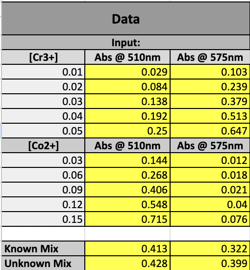
1. Obtain the absorbances of each diluted solution, the stock solution, and unknown solution.
2. For each ion, graph their absorbances at every dilution for both wavelengths 510 and 575 nm. Add in the line of best fit, and you should have a total of 4 lines.
3. These graphs will be used to determine the k values because the k value is equal to slope of the linear line of the best fit.
4. Knowing the k of each ion at 510 and 575 nm along with the absorbance of the unknowns will allow you to determine the concentration of Co2+ and Cr3+. Refer to the calculations below for an explanation why.

Calculations:

The following system of equations are used to find the concentrations. The highlighted variables are the unknown values you will be solving for. We get the following equations from the fact that absorbances are additive and that the absorbance of a solution is equal to its k value times its concentration (or A = KC). The graphs will provide you with the k values of each ion at each wavelength and the absorbance of the unknown is obtained from your lab data.

A₅₁₀ = A_{Cr 510} + A_{Co 510}

A₅₇₅ = A_{Cr 575} + A_{Co 575}

A₅₁₀ = K_{Cr 510} C_Cr + K_{Co 510} C_Co

A₅₇₅ = K_{Cr 575} C_Cr + K_{Co 575} C_Co

A₅₁₀ = absorbance of unknown at 510 nm

A₅₇₅ = absorbance of unknown at 575 nm

KCr₅₁₀ = k value of chromium at 510 nm

KCr₅₇₅ = k value of chromium at 575 nm

KCo₅₁₀ = k value of cobalt at 510 nm

KCo₅₇₅ = k value of cobalt at 575 nm

CCo = concentration of cobalt

CCr = concentration of chromium

Making the Graphs:

Example Graph	Lab 7 Computer Beer's Law - Student Edn..xlsx
Student Graph (MAKE A COPY OF THIS, FILL IT OUT WITH YOUR DATA TO MAKE YOUR GRAPHS)	Lab 7 Computer Beer's Law - Student Edn..xlsx

Procedure for Graphs:

1. Click “Student Graph” link above.

2. Click “File” then “Make a Copy.”

3. Following the instructions on YOUR BLANK COPY, add your experimental data obtained from the lab into the YELLOW HIGHLIGHTED BOXES. The rest of the sheet is set to run the calculations for you. Do NOT adjust the other parts. If you do, you can go back to the original and obtain the necessary functions to fix it.

 

4. The output part below your data input has data that is used in the calculations. Do not edit this part of the sheet.

5. Your graphs will automatically show up in this part of the sheet. The colors of the lines and dots on the graph are coordinated with the results on the left side. On the left, you will find each line’s respective slope value, standard deviation, and y-intercept. The #N/A is correct as there is no standard deviation for the y-intercept. Again, do not edit this part of the sheet.

6. Here are your results for the lab! The k-values correlate with the slopes of each line of best fit. For example, the k-value of Cr³⁺ at 510 nm is equal to the slope of that graph’s line of best fit. The standard deviation is also from each slope’s respective standard deviation. The data is simply consolidated to this table for your ease. Again, do not edit this part of the sheet.

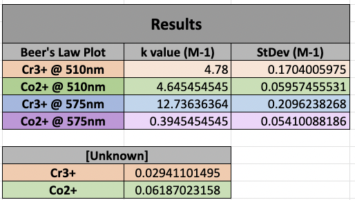
7. Finally, here are your unknown concentrations. They are calculated for you using the system of equations discussed on page 1. Again, do not edit this part of the sheet.