1.3: Experimental Details of Absorption spectroscopy
- Page ID
- 362578
\( \newcommand{\vecs}[1]{\overset { \scriptstyle \rightharpoonup} {\mathbf{#1}} } \)
\( \newcommand{\vecd}[1]{\overset{-\!-\!\rightharpoonup}{\vphantom{a}\smash {#1}}} \)
\( \newcommand{\id}{\mathrm{id}}\) \( \newcommand{\Span}{\mathrm{span}}\)
( \newcommand{\kernel}{\mathrm{null}\,}\) \( \newcommand{\range}{\mathrm{range}\,}\)
\( \newcommand{\RealPart}{\mathrm{Re}}\) \( \newcommand{\ImaginaryPart}{\mathrm{Im}}\)
\( \newcommand{\Argument}{\mathrm{Arg}}\) \( \newcommand{\norm}[1]{\| #1 \|}\)
\( \newcommand{\inner}[2]{\langle #1, #2 \rangle}\)
\( \newcommand{\Span}{\mathrm{span}}\)
\( \newcommand{\id}{\mathrm{id}}\)
\( \newcommand{\Span}{\mathrm{span}}\)
\( \newcommand{\kernel}{\mathrm{null}\,}\)
\( \newcommand{\range}{\mathrm{range}\,}\)
\( \newcommand{\RealPart}{\mathrm{Re}}\)
\( \newcommand{\ImaginaryPart}{\mathrm{Im}}\)
\( \newcommand{\Argument}{\mathrm{Arg}}\)
\( \newcommand{\norm}[1]{\| #1 \|}\)
\( \newcommand{\inner}[2]{\langle #1, #2 \rangle}\)
\( \newcommand{\Span}{\mathrm{span}}\) \( \newcommand{\AA}{\unicode[.8,0]{x212B}}\)
\( \newcommand{\vectorA}[1]{\vec{#1}} % arrow\)
\( \newcommand{\vectorAt}[1]{\vec{\text{#1}}} % arrow\)
\( \newcommand{\vectorB}[1]{\overset { \scriptstyle \rightharpoonup} {\mathbf{#1}} } \)
\( \newcommand{\vectorC}[1]{\textbf{#1}} \)
\( \newcommand{\vectorD}[1]{\overrightarrow{#1}} \)
\( \newcommand{\vectorDt}[1]{\overrightarrow{\text{#1}}} \)
\( \newcommand{\vectE}[1]{\overset{-\!-\!\rightharpoonup}{\vphantom{a}\smash{\mathbf {#1}}}} \)
\( \newcommand{\vecs}[1]{\overset { \scriptstyle \rightharpoonup} {\mathbf{#1}} } \)
\( \newcommand{\vecd}[1]{\overset{-\!-\!\rightharpoonup}{\vphantom{a}\smash {#1}}} \)
The absorption of light at a given \(λ\), can be used to measure concentration in solution. Electronic absorption spectra of solutes in liquid solution are generally broadened due to several factors including inhomogeneities in the local environment that do not average out – fluctuations that are too slow.
The characteristic timescale for the electronic transition is ~1 fs, while several fluctuations in the solvent are much slower ~ps. These local fluctuations of the solvent results in a “static inhomogeneity” of the absorption band. Thus rotational structure is not revealed and vibrational structure partially so (if at all) and are referred to as bands in the absorption.
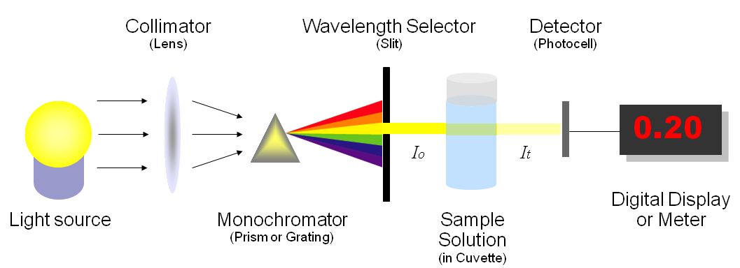
The amount of photons that goes through the cuvette and into the detector is dependent on the length of the cuvette and the concentration of the sample. Once you know the intensity of light after it passes through the cuvette, you can relate it to transmittance (\(T\)) (Figure \(\PageIndex{2}\)). Transmittance is the fraction of light that passes through the sample. This can be calculated using the equation:
\[\text{Transmittance} (T) = \dfrac{I_t}{I_o} \nonumber \]
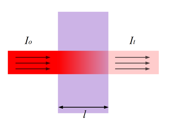
Most substances obey the Beer-Lambert law of absorption:
\[ A =\epsilon c l \nonumber \]
where absorbance (\(A\)) is related to transmission (\(T\)) via
\[ A = \log_{10}(T) \nonumber \]
where \(A\) is the absorbance, \(T_o\) is the incident light intensity, \(T\) is the transmitted light intensity, \(l\) is the thickness of the sample and \(c\) is the molar concentration of the solute and \(ε\) is the Extinction Coefficient or Molar Absorptivity of the solute at the probed wavelength.
\(ε\) is a function of \(λ\) and thus is \(A\). A plot of \(A\) vs. \(λ\) of \(ε\) vs. \(λ\) is absorption the absorption spectrum. If the Beers-Lambert law is obeyed, then \(A(λ)\) is proportional to \(c\) and \(c\) can be determined if \(ε (λ)\) is known - i.e., quantitative analysis.
This is the basis of quantitative analysis by spectrophotometry. Testing the Beers-Lambert law:
\[ε (λ) = \dfrac{A(λ)}{c} \nonumber \]
If we assume a 1 cm cell so \(l\) is 1.
If the \(A(λ)/c\) ratio is constant at different concentrations than the Beers-Lambert law is obeyed and \(ε(λ)\) is given by this ratio. Consequently,
\[c= \dfrac{A(λ)_{1 \,cm}}{εlc} \nonumber \]
The units of \(ε\) are in liters mol-1 cm-1. \(l\) is by convention in cm.
Determining concentrations from spectra
Simultaneous determination of concentration of two simultaneously present absorbers (\(B\) and \(C\)) is possible from measuring @ two wavelengths, \(λ_1\) and \(λ_2\). In a 1 cm pathlength cell,
\[A_1=A(λ_1) =ε_b(λ_1) c_b+ ε_c(λ_1)c_c \nonumber \]
\[A_2=A(λ_2) =ε_b(λ_2) c_b+ ε_c(λ_2)c_c \nonumber \]
Simultaneous solutions of this linear system of equations are possible provided
\[\operatorname{det}\left|\begin{array}{ll}
\varepsilon_{B}\left(\lambda_{1}\right) & \varepsilon_{C}\left(\lambda_{1}\right) \\
\varepsilon_{B}\left(\lambda_{2}\right) & \varepsilon_{C}\left(\lambda_{2}\right)
\end{array}\right| \neq 0 \nonumber \]
If this is 0 (or close to it), then the equations are linearly dependent and no unique solution for \(c_b\) and \(c_b\) possible. The wavelengths, \(λ_1\) and \(λ_2\) should be chosen to yield a large value for the determinant.
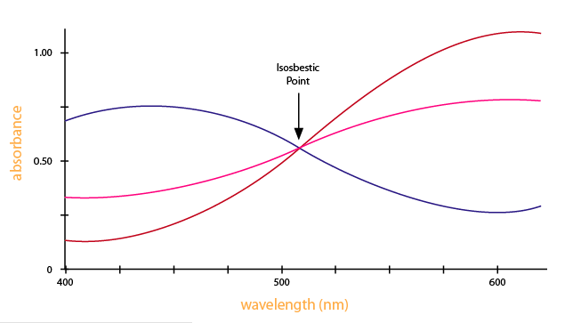
Isosbestic Points
If there are only two species present in solution that absorbs, \(S\) and \(ES\), for instance, and they have overlapping spectra, there will be at least one wavelength, \(λ_o\), where \[ε_S(λ_o)= ε_{ES}(λ_o). \nonumber \]
The absorbance @ \(λ_o\) will be constant irrespective of the condition of the sample (in equilibrium or out of equilibrium) assuming constant sum of populations.
\[\begin{align*} A(λ)_o) &= x ε_S(λ_o) + y ε_S(λ_o) \\[4pt] &= (x+y) ε_S(λ_o) \end{align*} \nonumber \]
\(λ_o\) defines an isobestic point. If we know the spectrum of \(S\) and \(ES\), \(λ_o\) can be determined.
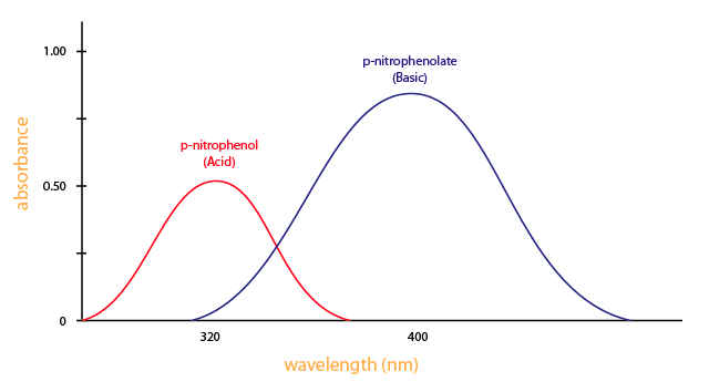
You need a spectrometer to produce a variety of wavelengths because different compounds absorb best at different wavelengths. For example, p-nitrophenol (acid form) has the maximum absorbance at approximately 320 nm and p-nitrophenolate (basic form) absorbs best at 400 nm (Figure \(\PageIndex{3}\)).
Looking at the graph that measures absorbance and wavelength, an isosbestic point can also be observed. An isosbestic point is the wavelength in which the absorbance of two or more species are the same. The appearance of an isosbestic point in a reaction demonstrates that an intermediate is NOT required to form a product from a reactant. Figure \(\PageIndex{4}\) shows an example of an isosbestic point.