1: Electricity and Units

Electricity is part of our every day world and yet most of us have very little understanding of what electricity is.  This chapter is more of a reference chapter and you should come back to it as needed.

Electricity is typically considered to be the flow of electric charge, although it can also be referred to stored or accumulated charge, usually in the form of electrons, and it can be produced by other sources of energy (coal, natural gas, solar energy, etc..) and harnessed to power electronic devices, provide lighting and do various forms of work. The coulomb (C) is the fundamental unit of charge and the flow of electricity is measured in amperes (C/s). Voltage (V) is the electric potential energy per unit charge (coulomb) and current times voltages is the power that is measured in watts (W). An electric circuit represents the path the current flows as the charge moves from a high to a low potential.

The flow of electric current can cause some confusion to chemistry students who understand that it is the electron that typically flows in a circuit, which is a negative charged particle and thus flows to the positive (high potential), so in engineering circuits the direction of flow is that for which a positive particle would flow.

We will start our discussion of electricity from the perspective of the units of measurement, noting that the way the SI base units that can describe all measurable phenomena were radically changed in 2019 to be based on 7 immutable constants (Chem 1402 Units of Measurement), which are defined (exact) numbers.

SI Units

All measurable phenomena can be measured with the 7 SI (Système international d'unités) base units as defined by the Bureau international des poids et mesures (BIPM). These base units are:

1. meter (length)
2. kilogram (mass)
3. second (time)
4. Kelvin (absolute temperature)
5. mole (quantity)
6. ampere (electric current)
7. candela (luminous intensity)

 

In 2019 the way these units were defined was changed to be based on seven immutable constants of nature (figure 1).

Figure \(\PageIndex{1}\): Seven Immutable Constants that SI base units are defined by. (Stoughton/NIST)

Coulomb (C): Unit of Charge (q)

The Coulomb (C) is defined by the charge of an elementary particle (electron, or positron) where the charge is defined by:

\[ \text{Charge of an electron } (e^-) \equiv -1.602176634x10^{-19}C \\ \text{Charge of a positron } (e^+) \equiv 1.602176634x10^{-19}C \]

Therefore:

\[\text{1 Coulomb (C)} =\frac{1}{1.602176634x10^{-19}C} = \text{the charge of } 6.241509074 x 10^{18} \text{ electrons or positrons}\]

In electronics the symbol q is used to denote charge of an individual particle and C is the unit. As electrons and not positrons are what commonly flow in electric circuits we will implicitly refer to an electron as something with a negative charge, without explicitly stating so.

Faraday (F): Charge of a mole of electrons (Q)

Multiplying the SI constant of the charge of an electron (e) with that of quantity (the mole, N_{A ,} Avagaordo's number) gives us the charge of a mole of electrons, which is Faraday's constant:

\[1F \equiv 1(N_A)(e)=(\frac{6.02214076 x10^{23} electrons}{mole \; electrons})\frac{1.602176634x10^{-19}C}{electron}=96,485.3321\frac{C}{mol \cdot electrons} \; \\ \; \\ \text{or more commonly} \\ \; \\ 1F=96,500 \frac{C}{mol electrons} \]

In electronics Q represents the total charge passing through a conductor over a period of time. A capacitor is a common electrical device that stores charge in the units of Faradays.

Ampere (A): Unit of Current (I)

We are often interested in the work done as charge flows, that is as charge flows over time, so if we divide the Si constant for charge by time we get the ampere.

\[1A \equiv \frac{1C}{1 \; sec}\]

96,500 amps = flow of one mole of electrons

In electronics the symbol I is used to denote current and amp is the unit

Volt (V): Unit of Electric Potential (V or \(\Delta\)E)

\[1 \text{Volt} \equiv \frac{1\text{ Joule}}{\text{Coulomb}} \text{, in terms of the base SI units: } 1V=\frac{kg \cdot m^2 \cdot s^{-2}}{A \cdot s}\]

Where the Joule is the unit of energy, which is the capacity to do work or transfer heat. This can be understood by comparing translational work to electronic work

• Translation Work: Energy (J) = W (work) = F \(\cdot\ \Delta x\)
  • Work done when a force displaces an object in a straight line
• Electronic Work: Energy (J) = W (work) = QV (or in chemistry we often write this as W = q \(\Delta\)E )
  • Work done when charge is moved across an electric potential
  • Current flows from high to low potential
  • Note, here W means work, but in electronics W is also the unit of electric power, the Watt.

so

\[ 1V=\frac{1J}{1C} \;\; and \;\; C=\frac{1J}{1V}\]

so we can relate work to Faraday's constant

\[1F \; = \; \frac{96,500C}{mole \; e^-} \; = \; \frac{96,500J}{V \cdot mole \; e^-} \] 

noting \(\Delta\)G is Gibbs free energy and n = moles electrons, we get the expression

\[ \Delta G = -nFE_{cell}^o =-QV\]

Where nF is the total charge of electrons (Q) and V is the electric potential drop.  For a spontaneous reactions the change in Gibbs free Energy is negative (\(\Delta\)G < 0) and this equates to a positive cell potential. This equation relates the sign of spontaneous flow from the perspective of free energy to that of electric potential as used in circuit diagrams, and a spontaneous flow will occur when V is positive (and (\(\Delta\)G is thus negative).

In electronics the Symbol V is used to denote electric potential, and it also the symbol of the unit for electric potential. That is, in V=IR we are saying the voltage equals the current times the resistance, but in 10 V, we are using it as a unit of measurement.

Watt (W): Unit of Electric Power (P)

Power is the rate at which work can be performed and has the unit of Watt

\[1W \; \equiv \; \frac{1J}{sec} \; = \; \frac{C \cdot V}{sec} \; = \; A \cdot V \]

In electronics the symbol P is used to denote power and Watt is the unit. Note, in the above equation V is being used as a unit, while in the next equation it is being used as a symbol for voltage

\[P=IV\]

IV Curves

A plot of the current as a function of the potential for an electric device is can provide information on. its power efficiency. This are often plotted to determine the best operating potential for a device.  If the device is an energy source, like a solar cell, than you want to operate at the highest point on the IV curve that has enough potential to drive the process you want to drive, as that produces the maximum amount of work (P_mp=I_mpV_mp).

Figure \(\PageIndex{1}\): Generic solar cell IB curve. (CC 3.0 Squirmymcphee, Wikimedia commons)

The above plot is a measure of the current as a function of the voltage as you apply a load and the maximum power the device can produce is when you operate at V_mp. Note, in this plot the current is the dependent variable and the voltage is the independent variable and the power is the product of these two (P=IV).  As you increase the voltage by adding a load the current drops.  V_oc is the open circuit voltage when no current flows (infinite load), and I_sc is the short circuit current when no load is applied

 

Watt Hour (Wh): Unit of Electric Energy (E)

\[1Wh \; \equiv \; 1W \cdot h \; = \; \frac{1J}{sec} \cdot 1h \; = \; 3600 Joules \]

Your electric meter reads in kWh or kiloWatt hours

Ohm (\(\Omega \)): Unit of Resistance(R) and Impedance(Z) to Electric Current Flow 

Resistance (R)

\[1\Omega \; \equiv \; \frac{1V}{1A} \]

Resistance is a measure of the resistance to the flow of electric current and has units of \(\Omega\). It is a property of the material with a conductor having a low resistance.  For a wire, the smaller the diameter the greater the resistance.  For a given voltage the greater the resistance the lower the current.  The relationship between resistance, voltage and current is given by Ohm's Law

\[\text{Ohm's Law  V=IR}\]

Impedance (Z)

In alternating circuits there are two other types resistance known as reactance, which occur due to the change in voltage (in contrast to the voltage itself) and the impedance (Z) is a function of both resistance (R) and the total Reactance (X_T)

\[ Z=\sqrt{R^2 +X_T^2} \] 

Reactance (X)

Reactance is the resistance to flow due to a change in the voltage, not the voltage itself and always occurs in AC circuits.  there are two types of reactance, inductive and capacitive.

Two Types

• X_L = Inductive Reactance - due to induced magnetic currents
• X_C = Capacitive Reactance - due to capacitor charge/discharge

Total Reactance (X_T)

• X_T = Total reactance
• X_T = X_L + X_C

 

Note

In this class we will be working predominantly with DC (Direct Current) circuits and will probably not have to deal with reactance and impedance.  It needs to be understood though that the \(\Omega\) is really the unit of Impedance, which has two components, the resistance and reactance. For DC circuits the reactance is often zero and so the impedance is the resistance, and this systems follow Ohm's Law.

V=IR

 

SI prefixes

Si prefixes are base 10 multipliers that allow on to quickly scale the magnitude of a number across a wide range of values. The following table gives the SI prefixes.

Table \(\PageIndex{1}\): SI prefixes.

Multiplier	Name	Abbreviation		Name	Multiplier
10^+30	quetta*	Q	q	quecto*	10^-30
10^+27	ronna*	R	r	ronto*	10^-27
10^+24	yotta	Y	y	yocto	10^-24
10^+21	zetta	Z	z	zepto	10^-21
10^+18	exa	E	a	atto	10^-18
10^+15	peta	P	f	femto	10^-15
10^+12	tera	T	p	pico	10^-12
10^+9	giga	G	n	nano	10^-9
10^+6	mega	M	m	micro	10^-6
10^+3	kilo	k	m	milli	10^-3
10^+2	hecto	h	c	centi	10^-2
10^+1	deca	da	d	deci	10^-1

*quetta, ronna, ronto & quecto were added in 2022 (https://www.bipm.org/en/cgpm-2022/resolution-3).

Use of SI prefixes

For real large or small numbers, the convention is to place a number with between 1 and 999 in front of the SI prefix, and use the appropriate prefix to show the value. So a memory stick with 1,200,000 bytes would be written as 1.2 Mbyte, not as 1,200 kbytes.

\[ \begin{align}  1,330,000,000m & =1 .33 \times 10^{9}m  =1.33 \; gigameters \nonumber \\  13,300,000,000m & =13.3 \times 10^{9}m =13.3 \;gigameters \nonumber \\ 133,000,000,000m & =133  \times 10^{9}m  = \; 133 \; gigameters \end{align}\]

SI prefixes and Calculators

What is the ENG key on scientific calculators?

Figure \(\PageIndex{8}\): Three display modes on TI 30 calculator.

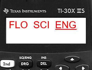
In Scientific Notation there is on digit to the left of the decimal, in Engineering notation there are 1, 2 or 3 digits to the left of the decimal, and you then use one of the Si prefixes that is of the magnitude 10³ⁿ.

The ENG key takes large or small numbers and expresses them as integer multiples of 10³ or 10^-3, effectively converting them to values that can be expressed with SI prefixes. If you type 1,200,000 into your calculator and press ENG, it gives 1.2 x 10⁶, so 1,200,000 bytes of memory on a memory stick would be 1.2 MBytes (you do not say 1,200 kBytes). If you try 0.12 and press ENG, it gives 120 x 10^-3, so 0.12g is 120 mg. So the ENG function quickly converts numbers to values that can easily be expressed with SI prefixes.

Note

Students are expected to be fluent in common SI prefixes as they are ubiqutous in electrical engineering.  You will be working with calibrated electrical components like M\(\Omega\) and K\(\Omega\) resistors and pF (Farad) capacitors, and need to know what the prefixes mean.

 

Tutorials

• SparkFun: What is Electricity
• SparkFun: Voltage, Current and Resistance
• SparkFun: Electric Power
• SparkFun: Polarity