3.8: Conformations of Monosubstituted Cyclohexanes

Objectives

After completing this section, you should be able to

1. account for the greater stability of the equatorial conformers of monosubstituted cyclohexanes compared to their axial counterparts, using the concept of 1,3‑diaxial interaction.
2. compare the gauche interactions in butane with the 1,3‑diaxial interactions in the axial conformer of methylcyclohexane.
3. arrange a given list of substituents in increasing or decreasing order of 1,3‑diaxial interactions.

Key Terms

Make certain that you can define, and use in context, the key term below.

• 1,3‑diaxial interaction

Study Notes

1,3-Diaxial interactions are steric interactions between an axial substituent located on carbon atom 1 of a cyclohexane ring and the hydrogen atoms (or other substituents) located on carbon atoms 3 and 5.

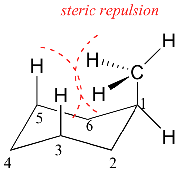
Be prepared to draw Newman-type projections for cyclohexane derivatives as the one shown for methylcyclohexane. Note that this is similar to the Newman projections from chapter 3 such as n-butane.

Newman projections of methylcyclohexane and n‑butane

Because axial bonds are parallel to each other, substituents larger than hydrogen experience greater steric crowding when they are oriented axial rather than equatorial. Consequently, substituted cyclohexanes will preferentially adopt conformations in which the larger substituents are in the equatorial orientation.

When the methyl group in the structure above occupies an axial position it experiences steric crowding by the two axial hydrogens located on the same side of the ring.

The conformation in which the methyl group is equatorial is more stable, and thus the ring flip equilibrium favors the conformation with the equatorial methyl group.

The relative steric hindrance experienced by different substituent groups oriented in an axial versus equatorial location on cyclohexane may be determined by the conformational equilibrium of the compound. The corresponding equilibrium constant is related to the energy difference between the conformers, and collecting such data allows us to evaluate the relative tendency of substituents to exist in an equatorial or axial location. Table 4.7.1 summarizes some of these free energy values (sometimes referred to as A values).

Looking at the energy values in this table, it is clear that as the size of the substituent increases, the 1,3-diaxial energy tends to increase, also.  Note that it is the size and not the molecular weight of the group that is important.

 

Table 4.7.1: A Selection of ΔG° Values for the Change from Axial to Equatorial Orientation of Substituents for Monosubstituted Cyclohexanes

Substituent	-ΔG°  (kcal/mol)	Substituent	-ΔG°  (kcal/mol)
\(\ce{CH_3\bond{-}}\)	1.7	\(\ce{O_2N\bond{-}}\)	1.1
\(\ce{CH_2H_5\bond{-}}\)	1.8	\(\ce{N#C\bond{-}}\)	0.2
\(\ce{(CH_3)_2CH\bond{-}}\)	2.2	\(\ce{CH_3O\bond{-}}\)	0.5
\(\ce{(CH_3)_3C\bond{-}}\)	\(\geq 5.0\)	\(\ce{HO_2C\bond{-}}\)	0.7
\(\ce{F\bond{-}}\)	0.3	\(\ce{H_2C=CH\bond{-}}\)	1.3
\(\ce{Cl\bond{-}}\)	0.5	\(\ce{C_6H_5\bond{-}}\)	3.0
\(\ce{Br\bond{-}}\)	0.5
\(\ce{I\bond{-}}\)	0.5

Chlorocyclohexane

This is an example of the next level of complexity, a mono-substituted cycloalkane.

 

Figure 4.7.3:  Chlorocyclohexane: simple hexagon and chair structures

 

The hexagon structure, Figure 4.7.3A. shows the basic "connectivity" of the atoms. This chemical has one Cl on the ring, and it does not matter where we show it.

The chair structure, Figure 4.7.3B, shows atom connectivity, and also the preferred conformation with the larger chlorine atom in the equatorial position. 

 

Helpful Hints

• Examine a physical model of cyclohexane and chlorocyclohexane, so that you can see the axial and equatorial positions. Common ball and stick models are fine for this. It should be easy to see that the three axial H on one side can get very near each other. If you do not have access to physical models, examining computer models can also be useful. When putting substituents on chair structures, I encourage you to use the four corner positions of the chair as much as possible. It is easier to see the axial and equatorial relationship at the corners.
• Draw both atoms attached to the ring carbons for clarity.  In Fig 4.7.3B the H atom that is on the same carbon as the Cl atom is shown. This is not necessary, but showing the H makes it clearer that the chlorine is in the equatorial position.

Exercises

Contributors

• Dr. Dietmar Kennepohl FCIC (Professor of Chemistry, Athabasca University)

• Prof. Steven Farmer (Sonoma State University)

>Robert Bruner (http://bbruner.org)

• Organic Chemistry With a Biological Emphasis by Tim Soderberg (University of Minnesota, Morris)