9.7: Molecular Orbitals Can Be Ordered According to Their Energies

The LCAO-MO method that we used for H₂⁺ can be applied qualitatively to homonuclear diatomic molecules to provide additional insight into chemical bonding. A more quantitative approach also is helpful, especially for more complicated situations, like heteronuclear diatomic molecules and polyatomic molecules. When two atoms are close enough for their valence orbitals to overlap significantly, the filled inner electron shells are largely unperturbed; hence they are often ignored in constructing molecular orbitals. This means that we can focus our attention on the molecular orbitals derived from valence atomic orbitals.

Molecular Orbitals Formed from ns Orbitals

The molecular orbitals diagrams formatted for the dihydrogen species are similar to the diagrams to any homonuclear diatomic molecule with two identical alkali metal atoms (Li₂ and Cs₂, for example) is shown in part (a) in Figure \(\PageIndex{1}\), where M represents the metal atom. Only two energy levels are important for describing the valence electron molecular orbitals of these species: a σ_ns bonding molecular orbital and a σ^*_ns antibonding molecular orbital. Because each alkali metal (M) has an ns¹ valence electron configuration, the M₂ molecule has two valence electrons that fill the σ_ns bonding orbital. As a result, a bond order of 1 is predicted for all homonuclear diatomic species formed from the alkali metals (Li₂, Na₂, K₂, Rb₂, and Cs₂). The general features of these M₂ diagrams are identical to the diagram for the H₂ molecule. Experimentally, all are found to be stable in the gas phase, and some are even stable in solution.

Figure \(\PageIndex{1}\): Molecular Orbital Energy-Level Diagrams for Alkali Metal and Alkaline Earth Metal Diatomic (\(M_2\)) Molecules. (a) For alkali metal diatomic molecules, the two valence electrons are enough to fill the σns (bonding) level, giving a bond order of 1. (b) For alkaline earth metal diatomic molecules, the four valence electrons fill both the \(σ_{ns}\) (bonding) and the \(σ_{ns}^*\) (nonbonding) levels, leading to a predicted bond order of 0. (CC BY-SA-NC; anonymous by request).

Similarly, the molecular orbital diagrams for homonuclear diatomic compounds of the alkaline earth metals (such as Be₂), in which each metal atom has an ns² valence electron configuration, resemble the diagram for the He₂ molecule. As shown in Figure \(\PageIndex{1b}\), this is indeed the case. All the homonuclear alkaline earth diatomic molecules have four valence electrons, which fill both the σ_ns bonding orbital and the σ_ns* antibonding orbital and give a bond order of 0. Thus Be₂, Mg₂, Ca₂, Sr₂, and Ba₂ are all expected to be unstable, in agreement with experimental data.In the solid state, however, all the alkali metals and the alkaline earth metals exist as extended lattices held together by metallic bonding. At low temperatures, \(Be_2\) is stable.

Example \(\PageIndex{1}\): Sodium Dimer Ion

Use a qualitative molecular orbital energy-level diagram to predict the valence electron configuration, bond order, and likely existence of the Na₂⁻ ion.

Given: chemical species

Asked for: molecular orbital energy-level diagram, valence electron configuration, bond order, and stability

Strategy

1. Combine the two sodium valence atomic orbitals to produce bonding and antibonding molecular orbitals. Draw the molecular orbital energy-level diagram for this system.
2. Determine the total number of valence electrons in the Na₂⁻ ion. Fill the molecular orbitals in the energy-level diagram beginning with the orbital with the lowest energy. Be sure to obey the Pauli principle and Hund’s rule while doing so.
3. Calculate the bond order and predict whether the species is stable.

Solution

A Because sodium has a [Ne]3s¹ electron configuration, the molecular orbital energy-level diagram is qualitatively identical to the diagram for the interaction of two 1s atomic orbitals.

B The Na₂⁻ ion has a total of three valence electrons (one from each Na atom and one for the negative charge), resulting in a filled σ_3s molecular orbital, a half-filled σ_3s* and a \( \left ( \sigma _{3s} \right )^{2}\left ( \sigma _{3s}^{\star } \right )^{1} \) electron configuration.

(CC BY-SA-NC; anonymous by request).

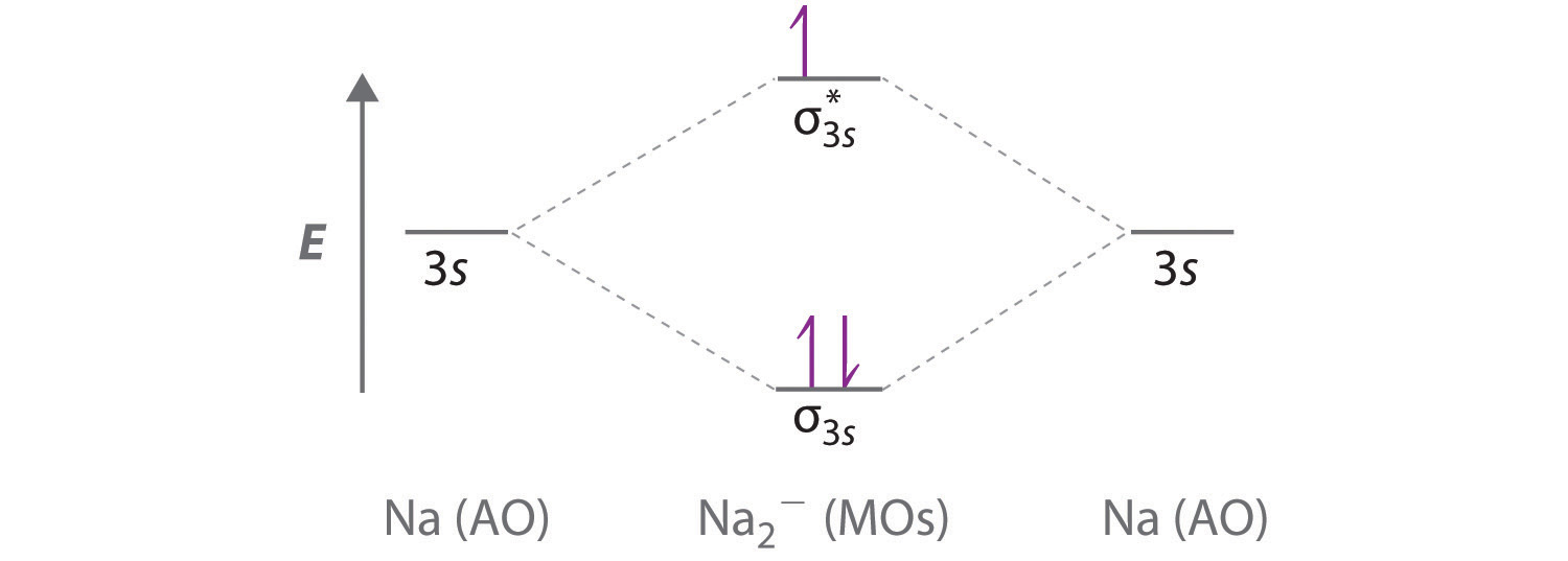
C The bond order is (2-1)÷2=1/2 With a fractional bond order, we predict that the Na₂⁻ ion exists but is highly reactive.

Exercise \(\PageIndex{1}\): Calcium Dimer Cation

Use a qualitative molecular orbital energy-level diagram to predict the valence electron configuration, bond order, and likely existence of the Ca₂⁺ ion.

Answer

Ca₂⁺ has a \( \left ( \sigma _{4s} \right )^{2}\left ( \sigma _{4s}^{\star } \right )^{1} \) electron configurations and a bond order of 1/2 and should exist.

Molecular Orbitals Formed from np Orbitals

Atomic orbitals other than ns orbitals can also interact to form molecular orbitals. Because individual p, d, and f orbitals are not spherically symmetrical, however, we need to define a coordinate system so we know which lobes are interacting in three-dimensional space. Recall that for each np subshell, for example, there are np_x, np_y, and np_z orbitals. All have the same energy and are therefore degenerate, but they have different spatial orientations.

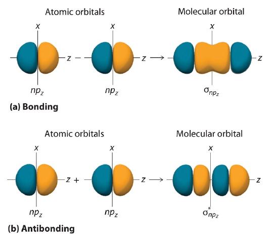
\[ \sigma _{np_{z}}=np_{z}\left ( A \right )-np_{z}\left ( B \right ) \label{9.7.1}\]

Just as with ns orbitals, we can form molecular orbitals from np orbitals by taking their mathematical sum and difference. When two positive lobes with the appropriate spatial orientation overlap, as illustrated for two np_z atomic orbitals in part (a) in Figure \(\PageIndex{2}\), it is the mathematical difference of their wave functions that results in constructive interference, which in turn increases the electron probability density between the two atoms. The difference therefore corresponds to a molecular orbital called a \( \sigma _{np_{z}} \) bonding molecular orbital because, just as with the σ orbitals discussed previously, it is symmetrical about the internuclear axis (in this case, the z-axis):

\[ \sigma _{np_{z}}=np_{z}\left ( A \right )-np_{z}\left ( B \right ) \label{9.7.2}\]

The other possible combination of the two np_z orbitals is the mathematical sum:

\[ \sigma _{np_{z}}=np_{z}\left ( A \right )+np_{z}\left ( B \right ) \label{9.7.3}\]

In this combination, shown in part (b) in Figure \(\PageIndex{2}\), the positive lobe of one np_z atomic orbital overlaps the negative lobe of the other, leading to destructive interference of the two waves and creating a node between the two atoms. Hence this is an antibonding molecular orbital. Because it, too, is symmetrical about the internuclear axis, this molecular orbital is called a \( \sigma _{np_{z}}=np_{z}\left ( A \right )-np_{z}\left ( B \right ) \) antibonding molecular orbital. Whenever orbitals combine, the bonding combination is always lower in energy (more stable) than the atomic orbitals from which it was derived, and the antibonding combination is higher in energy (less stable).

Figure \(\PageIndex{2}\): Formation of Molecular Orbitals from np_z Atomic Orbitals on Adjacent Atoms.(a) By convention, in a linear molecule or ion, the z-axis always corresponds to the internuclear axis, with +z to the right. As a result, the signs of the lobes of the np_z atomic orbitals on the two atoms alternate − + − +, from left to right. In this case, the σ (bonding) molecular orbital corresponds to the mathematical difference, in which the overlap of lobes with the same sign results in increased probability density between the nuclei. (b) In contrast, the σ* (antibonding) molecular orbital corresponds to the mathematical sum, in which the overlap of lobes with opposite signs results in a nodal plane of zero probability density perpendicular to the internuclear axis. (CC BY-SA-NC; anonymous by request).

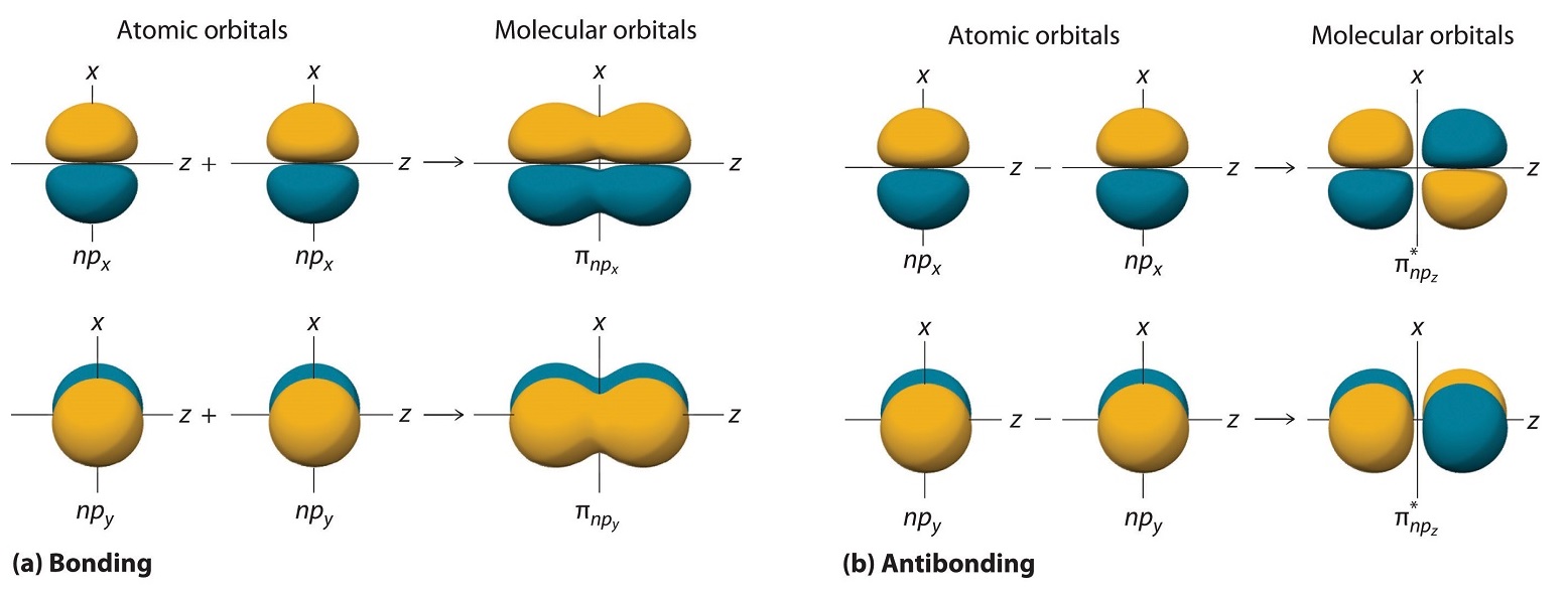
The remaining p orbitals on each of the two atoms, np_x and np_y, do not point directly toward each other. Instead, they are perpendicular to the internuclear axis. If we arbitrarily label the axes as shown in Figure \(\PageIndex{3}\), we see that we have two pairs of np orbitals: the two np_x orbitals lying in the plane of the page, and two np_y orbitals perpendicular to the plane. Although these two pairs are equivalent in energy, the np_x orbital on one atom can interact with only the np_x orbital on the other, and the np_y orbital on one atom can interact with only the np_y on the other. These interactions are side-to-side rather than the head-to-head interactions characteristic of σ orbitals. Each pair of overlapping atomic orbitals again forms two molecular orbitals: one corresponds to the arithmetic sum of the two atomic orbitals and one to the difference. The sum of these side-to-side interactions increases the electron probability in the region above and below a line connecting the nuclei, so it is a bonding molecular orbital that is called a pi (π) orbital (a bonding molecular orbital formed from the side-to-side interactions of two or more parallel np atomic orbitals). The difference results in the overlap of orbital lobes with opposite signs, which produces a nodal plane perpendicular to the internuclear axis; hence it is an antibonding molecular orbital, called a pi star (π*) orbital An antibonding molecular orbital formed from the difference of the side-to-side interactions of two or more parallel np atomic orbitals, creating a nodal plane perpendicular to the internuclear axis..

\[ \pi _{np_{x}}=np_{x}\left ( A \right )+np_{x}\left ( B \right ) \label{9.7.4}\]

\[ \pi ^{\star }_{np_{x}}=np_{x}\left ( A \right )-np_{x}\left ( B \right ) \label{9.7.5}\]

The two np_y orbitals can also combine using side-to-side interactions to produce a bonding \( \pi _{np_{y}} \) molecular orbital and an antibonding \( \pi _{np_{y}}^{\star } \) molecular orbital. Because the np_x and np_y atomic orbitals interact in the same way (side-to-side) and have the same energy, the \( \pi _{np_{x}} \) and \( \pi _{np_{y}} \)molecular orbitals are a degenerate pair, as are the \( \pi _{np_{x}}^{\star } \) and \( \pi _{np_{y}}^{\star } \) molecular orbitals.

Figure \(\PageIndex{3}\): Formation of π Molecular Orbitals from npx and npy Atomic Orbitals on Adjacent Atoms.(a) Because the signs of the lobes of both the npx and the npy atomic orbitals on adjacent atoms are the same, in both cases the mathematical sum corresponds to a π (bonding) molecular orbital. (b) In contrast, in both cases, the mathematical difference corresponds to a π* (antibonding) molecular orbital, with a nodal plane of zero probability density perpendicular to the internuclear axis. (CC BY-SA-NC; anonymous by request).

Energies for Homonuclear Diatomic Molecules

We now describe examples of systems involving period 2 homonuclear diatomic molecules, such as N₂, O₂, and F₂. When we draw a molecular orbital diagram for a molecule, there are four key points to remember:

1. The number of molecular orbitals produced is the same as the number of atomic orbitals used to create them.
2. As the overlap between two atomic orbitals increases, the difference in energy between the resulting bonding and antibonding molecular orbitals increases.
3. When two atomic orbitals combine to form a pair of molecular orbitals, the bonding molecular orbital is stabilized about as much as the antibonding molecular orbital is destabilized.
4. The interaction between atomic orbitals is greatest when they have the same energy.

Figure \(\PageIndex{4}\) is an energy-level diagram that can be applied to two identical interacting atoms that have three np atomic orbitals each. There are six degenerate p atomic orbitals (three from each atom) that combine to form six molecular orbitals, three bonding and three antibonding. The bonding molecular orbitals are lower in energy than the atomic orbitals because of the increased stability associated with the formation of a bond. Conversely, the antibonding molecular orbitals are higher in energy, as shown. The energy difference between the σ and σ* molecular orbitals is significantly greater than the difference between the two π and π* sets. The reason for this is that the atomic orbital overlap and thus the strength of the interaction are greater for a σ bond than a π bond, which means that the σ molecular orbital is more stable (lower in energy) than the π molecular orbitals.

Figure \(\PageIndex{4}\): The Relative Energies of the σ and π Molecular Orbitals Derived from np_x, np_y, and np_z Orbitals on Identical Adjacent Atoms. Because the two np_z orbitals point directly at each other, their orbital overlap is greater, so the difference in energy between the σ and σ* molecular orbitals is greater than the energy difference between the π and π* orbitals. (CC BY-SA-NC; anonymous by request).

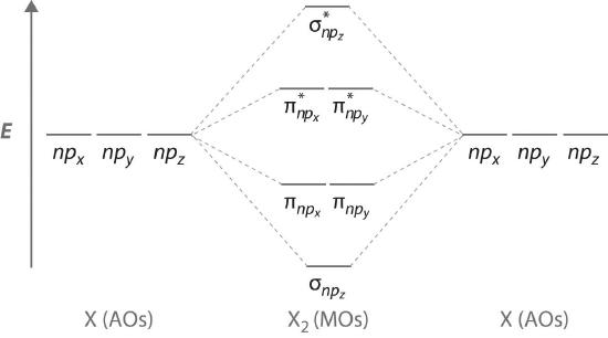
The number of molecular orbitals is always equal to the total number of atomic orbitals we started with.

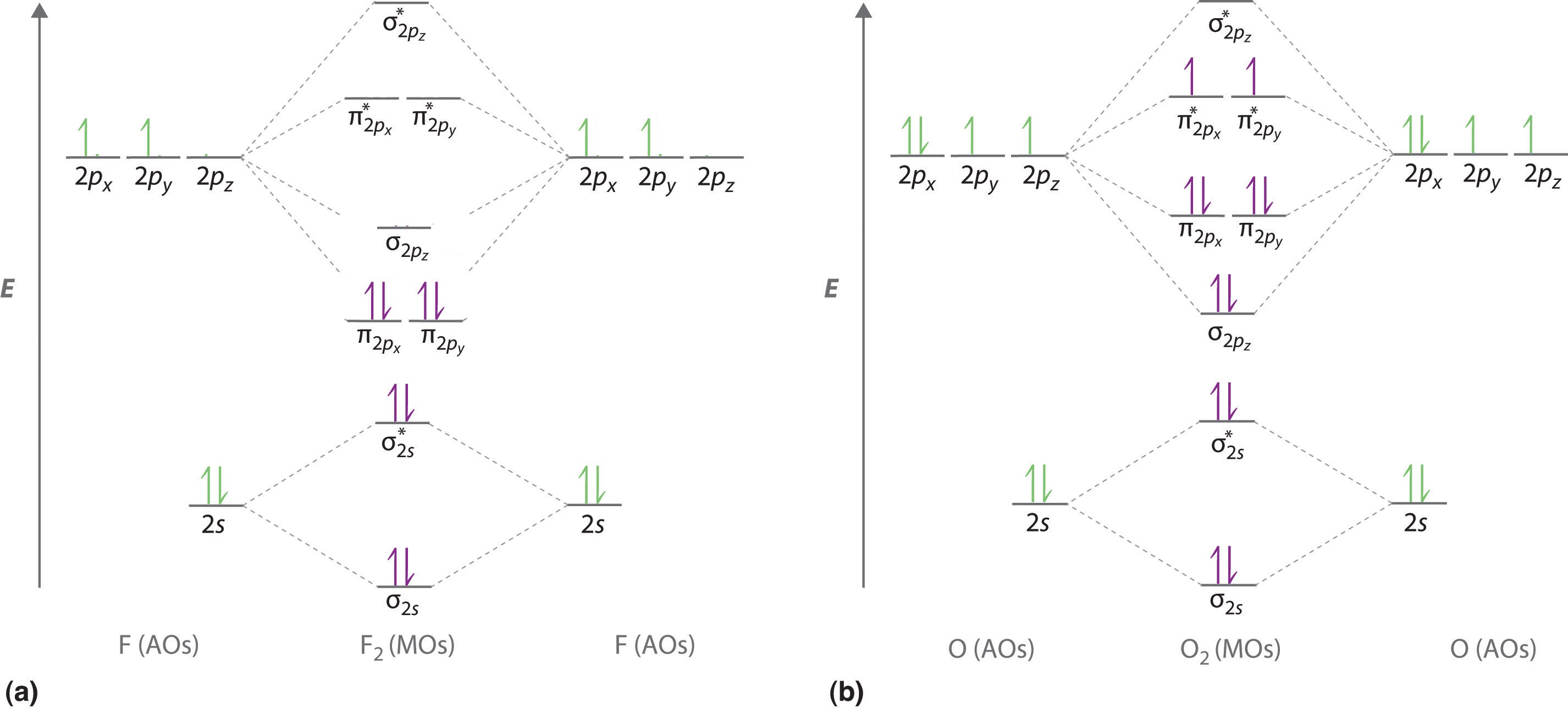
We illustrate how to use these points by constructing a molecular orbital energy-level diagram for F₂. We use the diagram in Figure \(\PageIndex{5a}\); the n = 1 orbitals (σ_1s and σ_1s*) are located well below those of the n = 2 level and are not shown. As illustrated in the diagram, the σ_2s and σ_2s* molecular orbitals are much lower in energy than the molecular orbitals derived from the 2p atomic orbitals because of the large difference in energy between the 2s and 2p atomic orbitals of fluorine. The lowest-energy molecular orbital derived from the three 2p orbitals on each F is \( \sigma _{2p_{z}} \) and the next most stable are the two degenerate orbitals, \( \pi _{2p_{x}} \) and \( \pi _{2p_{y}} \). For each bonding orbital in the diagram, there is an antibonding orbital, and the antibonding orbital is destabilized by about as much as the corresponding bonding orbital is stabilized. As a result, the \( \sigma ^{\star }_{2p_{z}} \) orbital is higher in energy than either of the degenerate \( \pi _{2p_{x}}^{\star } \) and \( \pi _{2p_{y}}^{\star } \) orbitals. We can now fill the orbitals, beginning with the one that is lowest in energy.

Each fluorine has 7 valence electrons, so there are a total of 14 valence electrons in the F₂ molecule. Starting at the lowest energy level, the electrons are placed in the orbitals according to the Pauli principle and Hund’s rules. Two electrons each fill the σ_2s and σ_2s* orbitals, 2 fill the \( \sigma _{2p_{z}} \) orbital, 4 fill the two degenerate π orbitals, and 4 fill the two degenerate π^* orbitals, for a total of 14 electrons.

Figure \(\PageIndex{5}\): Molecular Orbital Energy-Level Diagrams for Homonuclear Diatomic Molecules.(a) For C₂, with 8 valence electrons (4 from each F atom). This diagram shows 6 electrons in bonding orbitals and 2 in antibonding orbitals, resulting in a bond order of 2. (b) For O₂, with 12 valence electrons (6 from each O atom), there are only 2 electrons to place in the \( \left ( \pi ^{\star }_{np_{x}},\; \pi ^{\star }_{np_{y}} \right ) \) pair of orbitals. Hund’s rule dictates that one electron occupies each orbital, and their spins are parallel, giving the O₂ molecule two unpaired electrons. This diagram shows 8 electrons in bonding orbitals and 4 in antibonding orbitals, resulting in a predicted bond order of 2. (CC BY-SA-NC; anonymous by request).

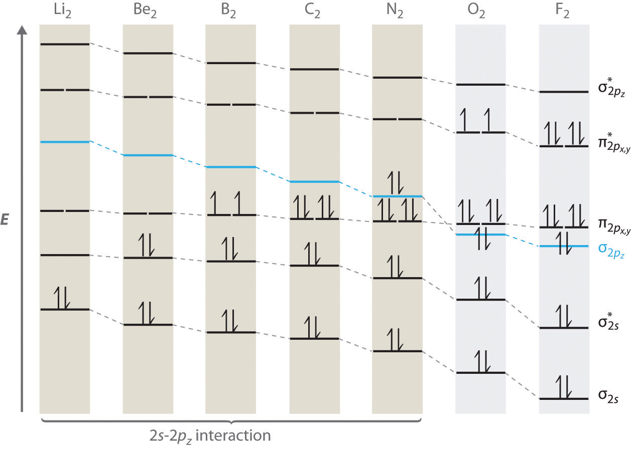
For period 2 diatomic molecules to the left of N₂ in the periodic table, a slightly different molecular orbital energy-level diagram is needed because the \( \sigma _{2p_{z}} \) molecular orbital is slightly higher in energy than the degenerate \( \pi ^{\star }_{np_{x}} \) and \( \pi ^{\star }_{np_{y}} \) orbitals. The difference in energy between the 2s and 2p atomic orbitals increases from Li₂ to F₂ due to increasing nuclear charge and poor screening of the 2s electrons by electrons in the 2p subshell. The bonding interaction between the 2s orbital on one atom and the 2p_z orbital on the other is most important when the two orbitals have similar energies. This interaction decreases the energy of the σ_2s orbital and increases the energy of the \( \sigma _{2p_{z}} \) orbital. Thus for Li₂, Be₂, B₂, C₂, and N₂, the \( \sigma _{2p_{z}} \) orbital is higher in energy than the \( \sigma _{3p_{z}} \) orbitals, as shown in Figure \(\PageIndex{6}\). Experimentally, the energy gap between the ns and np atomic orbitals increases as the nuclear charge increases (Figure \(\PageIndex{6}\)). Thus for example, the \( \sigma _{2p_{z}} \) molecular orbital is at a lower energy than the \( \pi _{2p_{x,y}} \) pair.

Figure \(\PageIndex{6}\): Molecular Orbital Energy-Level Diagrams for the Diatomic Molecules of the Period 2 Elements. Unlike earlier diagrams, only the molecular orbital energy levels for the molecules are shown here. For simplicity, the atomic orbital energy levels for the component atoms have been omitted. For Li₂ through N₂, the \( \sigma _{2p_{z}} \) orbital is higher in energy than the \( \pi _{2p_{x,y}} \) orbitals. In contrast, the \( \sigma _{2p_{z}} \) orbital is lower in energy than the \( \pi _{2p_{x,y}} \) orbitals for O₂ and F₂ due to the increase in the energy difference between the 2s and 2p atomic orbitals as the nuclear charge increases across the row. (CC BY-SA-NC; anonymous by request).

Example \(\PageIndex{2}\): Diatomic Sulfur

Use a qualitative molecular orbital energy-level diagram to predict the electron configuration, the bond order, and the number of unpaired electrons in S₂, a bright blue gas at high temperatures.

Given: chemical species

Asked for: molecular orbital energy-level diagram, bond order, and number of unpaired electrons

Strategy:

1. Write the valence electron configuration of sulfur and determine the type of molecular orbitals formed in S₂. Predict the relative energies of the molecular orbitals based on how close in energy the valence atomic orbitals are to one another.
2. Draw the molecular orbital energy-level diagram for this system and determine the total number of valence electrons in S₂.
3. Fill the molecular orbitals in order of increasing energy, being sure to obey the Pauli principle and Hund’s rule.
4. Calculate the bond order and describe the bonding.

Solution:

A Sulfur has a [Ne]3s²3p⁴ valence electron configuration. To create a molecular orbital energy-level diagram similar to those in Figures \(\PageIndex{6}\) and \(\PageIndex{7}\), we need to know how close in energy the 3s and 3p atomic orbitals are because their energy separation will determine whether the \( \pi _{3p_{x,y}} \) or the \( \sigma _{3p_{z}} \)> molecular orbital is higher in energy. Because the ns–np energy gap increases as the nuclear charge increases, the \( \sigma _{3p_{z}} \) molecular orbital will be lower in energy than the \( \pi _{3p_{x,y}} \) pair.

B The molecular orbital energy-level diagram is as follows:

(CC BY-SA-NC; anonymous by request).

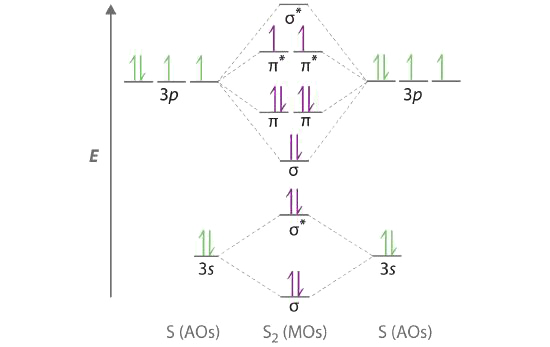
Each sulfur atom contributes 6 valence electrons, for a total of 12 valence electrons.

C Ten valence electrons are used to fill the orbitals through \( \pi _{3p_{x}} \) and \( \pi _{3p_{y}} \), leaving 2 electrons to occupy the degenerate \( \pi ^{\star }_{3p_{x}} \) and \( \pi ^{\star }_{3p_{y}} \) pair. From Hund’s rule, the remaining 2 electrons must occupy these orbitals separately with their spins aligned. With the numbers of electrons written as superscripts, the electron configuration of S₂ is \( \left ( \sigma _{3s} \right )^{2}\left ( \sigma ^{\star }_{3s} \right )^{2}\left ( \sigma _{3p_{z}} \right )^{2}\left ( \pi _{3p_{x,y}} \right )^{4}\left ( \pi _{3p ^{\star }_{x,y}} \right )^{2} \) with 2 unpaired electrons. The bond order is (8 − 4) ÷ 2 = 2, so we predict an S=S double bond.

Exercise \(\PageIndex{2}\)

Use a qualitative molecular orbital energy-level diagram to predict the electron configuration, the bond order, and the number of unpaired electrons in the peroxide ion (O₂²⁻).

Answer

\( \left ( \sigma _{2s} \right )^{2}\left ( \sigma ^{\star }_{2s} \right )^{2}\left ( \sigma _{2p_{z}} \right )^{2}\left ( \pi _{2p_{x,y}} \right )^{4}\left ( \pi _{2p ^{\star }_{x,y}} \right )^{4} \) bond order of 1; no unpaired electrons

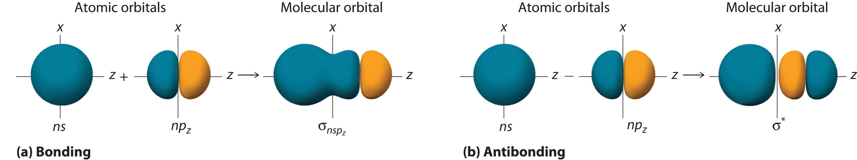
Molecular Orbitals Formed from ns with np Orbitals

Although many combinations of atomic orbitals form molecular orbitals, we will discuss only one other interaction: an ns atomic orbital on one atom with an np_z atomic orbital on another. As shown in Figure \(\PageIndex{7}\), the sum of the two atomic wave functions (ns + np_z) produces a σ bonding molecular orbital. Their difference (ns − np_z) produces a σ* antibonding molecular orbital, which has a nodal plane of zero probability density perpendicular to the internuclear axis.

Figure \(\PageIndex{7}\): Formation of Molecular Orbitals from an ns Atomic Orbital on One Atom and an np_z Atomic Orbital on an Adjacent Atom.(a) The mathematical sum results in a σ (bonding) molecular orbital, with increased probability density between the nuclei. (b) The mathematical difference results in a σ* (antibonding) molecular orbital, with a nodal plane of zero probability density perpendicular to the internuclear axis. (CC BY-SA-NC; anonymous by request).