
9.2: The H₂⁺ Prototypical Species
- Page ID
- 210853
\( \newcommand{\vecs}[1]{\overset { \scriptstyle \rightharpoonup} {\mathbf{#1}} } \)
\( \newcommand{\vecd}[1]{\overset{-\!-\!\rightharpoonup}{\vphantom{a}\smash {#1}}} \)
\( \newcommand{\id}{\mathrm{id}}\) \( \newcommand{\Span}{\mathrm{span}}\)
( \newcommand{\kernel}{\mathrm{null}\,}\) \( \newcommand{\range}{\mathrm{range}\,}\)
\( \newcommand{\RealPart}{\mathrm{Re}}\) \( \newcommand{\ImaginaryPart}{\mathrm{Im}}\)
\( \newcommand{\Argument}{\mathrm{Arg}}\) \( \newcommand{\norm}[1]{\| #1 \|}\)
\( \newcommand{\inner}[2]{\langle #1, #2 \rangle}\)
\( \newcommand{\Span}{\mathrm{span}}\)
\( \newcommand{\id}{\mathrm{id}}\)
\( \newcommand{\Span}{\mathrm{span}}\)
\( \newcommand{\kernel}{\mathrm{null}\,}\)
\( \newcommand{\range}{\mathrm{range}\,}\)
\( \newcommand{\RealPart}{\mathrm{Re}}\)
\( \newcommand{\ImaginaryPart}{\mathrm{Im}}\)
\( \newcommand{\Argument}{\mathrm{Arg}}\)
\( \newcommand{\norm}[1]{\| #1 \|}\)
\( \newcommand{\inner}[2]{\langle #1, #2 \rangle}\)
\( \newcommand{\Span}{\mathrm{span}}\) \( \newcommand{\AA}{\unicode[.8,0]{x212B}}\)
\( \newcommand{\vectorA}[1]{\vec{#1}} % arrow\)
\( \newcommand{\vectorAt}[1]{\vec{\text{#1}}} % arrow\)
\( \newcommand{\vectorB}[1]{\overset { \scriptstyle \rightharpoonup} {\mathbf{#1}} } \)
\( \newcommand{\vectorC}[1]{\textbf{#1}} \)
\( \newcommand{\vectorD}[1]{\overrightarrow{#1}} \)
\( \newcommand{\vectorDt}[1]{\overrightarrow{\text{#1}}} \)
\( \newcommand{\vectE}[1]{\overset{-\!-\!\rightharpoonup}{\vphantom{a}\smash{\mathbf {#1}}}} \)
\( \newcommand{\vecs}[1]{\overset { \scriptstyle \rightharpoonup} {\mathbf{#1}} } \)
\( \newcommand{\vecd}[1]{\overset{-\!-\!\rightharpoonup}{\vphantom{a}\smash {#1}}} \)
\(\newcommand{\avec}{\mathbf a}\) \(\newcommand{\bvec}{\mathbf b}\) \(\newcommand{\cvec}{\mathbf c}\) \(\newcommand{\dvec}{\mathbf d}\) \(\newcommand{\dtil}{\widetilde{\mathbf d}}\) \(\newcommand{\evec}{\mathbf e}\) \(\newcommand{\fvec}{\mathbf f}\) \(\newcommand{\nvec}{\mathbf n}\) \(\newcommand{\pvec}{\mathbf p}\) \(\newcommand{\qvec}{\mathbf q}\) \(\newcommand{\svec}{\mathbf s}\) \(\newcommand{\tvec}{\mathbf t}\) \(\newcommand{\uvec}{\mathbf u}\) \(\newcommand{\vvec}{\mathbf v}\) \(\newcommand{\wvec}{\mathbf w}\) \(\newcommand{\xvec}{\mathbf x}\) \(\newcommand{\yvec}{\mathbf y}\) \(\newcommand{\zvec}{\mathbf z}\) \(\newcommand{\rvec}{\mathbf r}\) \(\newcommand{\mvec}{\mathbf m}\) \(\newcommand{\zerovec}{\mathbf 0}\) \(\newcommand{\onevec}{\mathbf 1}\) \(\newcommand{\real}{\mathbb R}\) \(\newcommand{\twovec}[2]{\left[\begin{array}{r}#1 \\ #2 \end{array}\right]}\) \(\newcommand{\ctwovec}[2]{\left[\begin{array}{c}#1 \\ #2 \end{array}\right]}\) \(\newcommand{\threevec}[3]{\left[\begin{array}{r}#1 \\ #2 \\ #3 \end{array}\right]}\) \(\newcommand{\cthreevec}[3]{\left[\begin{array}{c}#1 \\ #2 \\ #3 \end{array}\right]}\) \(\newcommand{\fourvec}[4]{\left[\begin{array}{r}#1 \\ #2 \\ #3 \\ #4 \end{array}\right]}\) \(\newcommand{\cfourvec}[4]{\left[\begin{array}{c}#1 \\ #2 \\ #3 \\ #4 \end{array}\right]}\) \(\newcommand{\fivevec}[5]{\left[\begin{array}{r}#1 \\ #2 \\ #3 \\ #4 \\ #5 \\ \end{array}\right]}\) \(\newcommand{\cfivevec}[5]{\left[\begin{array}{c}#1 \\ #2 \\ #3 \\ #4 \\ #5 \\ \end{array}\right]}\) \(\newcommand{\mattwo}[4]{\left[\begin{array}{rr}#1 \amp #2 \\ #3 \amp #4 \\ \end{array}\right]}\) \(\newcommand{\laspan}[1]{\text{Span}\{#1\}}\) \(\newcommand{\bcal}{\cal B}\) \(\newcommand{\ccal}{\cal C}\) \(\newcommand{\scal}{\cal S}\) \(\newcommand{\wcal}{\cal W}\) \(\newcommand{\ecal}{\cal E}\) \(\newcommand{\coords}[2]{\left\{#1\right\}_{#2}}\) \(\newcommand{\gray}[1]{\color{gray}{#1}}\) \(\newcommand{\lgray}[1]{\color{lightgray}{#1}}\) \(\newcommand{\rank}{\operatorname{rank}}\) \(\newcommand{\row}{\text{Row}}\) \(\newcommand{\col}{\text{Col}}\) \(\renewcommand{\row}{\text{Row}}\) \(\newcommand{\nul}{\text{Nul}}\) \(\newcommand{\var}{\text{Var}}\) \(\newcommand{\corr}{\text{corr}}\) \(\newcommand{\len}[1]{\left|#1\right|}\) \(\newcommand{\bbar}{\overline{\bvec}}\) \(\newcommand{\bhat}{\widehat{\bvec}}\) \(\newcommand{\bperp}{\bvec^\perp}\) \(\newcommand{\xhat}{\widehat{\xvec}}\) \(\newcommand{\vhat}{\widehat{\vvec}}\) \(\newcommand{\uhat}{\widehat{\uvec}}\) \(\newcommand{\what}{\widehat{\wvec}}\) \(\newcommand{\Sighat}{\widehat{\Sigma}}\) \(\newcommand{\lt}{<}\) \(\newcommand{\gt}{>}\) \(\newcommand{\amp}{&}\) \(\definecolor{fillinmathshade}{gray}{0.9}\)Molecular orbital theory is a conceptual extension of the orbital model, which was so successfully applied to atomic structure. As was once playfully remarked, "a molecule is nothing more than an atom with more nuclei." This may be overly simplistic, but we do attempt, as far as possible, to exploit analogies with atomic structure. Our understanding of atomic orbitals began with the exact solutions of a prototype problem – the hydrogen atom. We will begin our study of homonuclear diatomic molecules beginning with another exactly solvable prototype, the hydrogen molecule-ion \(H_{2}^{+}\).
The Hydrogen Molecular Ion
The simplest conceivable molecule would be made of two protons and one electron, namely \(H_{2}^{+}\). This species actually has a transient existence in electrical discharges through hydrogen gas and has been detected by mass spectrometry and it also has been detected in outer space. The Schrödinger equation for \(H_{2}^{+}\) can be solved exactly within the Born-Oppenheimer approximation (i.e., fixed nuclei). This ion consists of two protons held together by the electrostatic force of a single electron. Clearly the two protons, two positive charges, repeal each other. The protons must be held together by an attractive Coulomb force that opposes the repulsive Coulomb force. A negative charge density between the two protons would produce the required counter-acting Coulomb force needed to pull the protons together. So intuitively, to create a chemical bond between two protons or two positively charged nuclei, a high density of negative charge between them is needed. We expect the molecular orbitals that we find to reflect this intuitive notion.
The electronic Hamiltonian for H2+ is
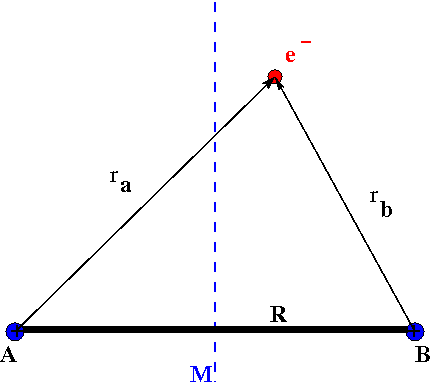
\[\hat {H}_{elec} (r, R) = -\dfrac {\hbar ^2}{2m} \nabla ^2 - \dfrac {e^2}{4 \pi \epsilon _0 r_A} - \dfrac {e^2}{4 \pi \epsilon _0 r_B} + \dfrac {e^2}{4 \pi \epsilon _0 R} \label{9.2.1}\]
where
- \(r_A\) and \(r_B\) are the distances electron from the \(A\) and \(B\) hydrogen nuclei, respectively and
- \(R\) is the distance between the two protons.
Although the Schrödinger equation for H2+ can be solved exactly (albeit within the Born-Oppenheimer approximation where the nuclei are fixed) because there is only one electron, we will develop approximate solutions in a manner applicable to other diatomic molecules that have more than one electron.
Linear Combination of Atomic Orbitals
For the case where the protons in H2+ are infinitely far apart, we have a hydrogen atom and an isolated proton when the electron is near one proton or the other. The electronic wavefunction would just be \(1s_A(r)\) or \(1s_B(r)\) depending upon which proton, labeled \(A\) or \(B\), the electron is near. Here \(1s_A\) denotes a 1s hydrogen atomic orbital with proton A serving as the origin of the spherical polar coordinate system in which the position r of the electron is specified. Similarly \(1s_B\) has proton B as the origin. A useful approximation for the molecular orbital when the protons are close together therefore is a linear combination of the two atomic orbitals. The general method of using
\[\psi (r) = C_A 1s_A (r) + C_B1s_B (r) \label{9.2.2}\]
i.e. of finding molecular orbitals as linear combinations of atomic orbitals is called the Linear Combination of Atomic Orbitals - Molecular Orbital (LCAO-MO) Method. In this case we have two basis functions in our basis set, the hydrogenic atomic orbitals 1sA and 1sB.
The LCAO approximation is an example of the linear variational method discussed previously with the true molecular orbital wavefunction approximated as an expansion of a basis set of atomic orbitals on each atom of the molecule with variable coefficients that can be optimized (e.g., via the secular equations). As discussed previously, the number of wavefunctions (solutions) extracted from solving the secular determinant is equal the number of elements in the expansion. So for the expansion in Equation \ref{9.2.2} with two atomic orbitals contributing result in two molecule orbitals.
This method yields a approximate picture of the molecular orbitals in a molecules. The figure below shows two atoms approaching along the axis of one of their \(2p\) states. In the top row, the two lobes facing one another have the same sign; in the bottom row they have opposite sign. These are two different linear combinations of the same two atomic states, on different atoms and with difference phases (i.e., signs of \(C_A\) vs. \(C_B\) in the expansion). In the first example, the electron density increases between the nuclei and in the second example, a very steep-sided node between the two nuclei causes all the probability density to face away from the atom opposite.

For H2+, the simplest molecule, the starting function is given by Equation \(\ref{9.2.2}\). We must determine the values for the coefficients, CA and CB. We could use the variational method to find a value for these coefficients, but for the case of H2+ evaluating these coefficients is easy. Since the two protons are identical, the probability that the electron is near A must equal the probability that the electron is near B. These probabilities are given by \(|C_A|^2\) and \(|C_B|^2\), respectively. Consider two possibilities that satisfy the condition \(|C_A|^2 = |C_B|^2\); namely, \(C_A = C_B = C_{+}\) and \(C_A = -C_B = C_{-}\). These two cases produce two molecular orbitals:
\[\psi _+ = C_+(1s_A + 1s_B) \label{9.2.3a}\]
\[\psi _{-} = C_{-}(1s_A - 1s_B) \label{9.2.3b}\]
The probability density for finding the electron at any point in space is given by \(|{\psi}^2|\) and the electronic charge density is just \(|e{\psi}^2|\). The important difference between \(\psi _+\) and \(\psi _{-}\) is that the charge density for \(\psi _+\) is enhanced (Figure \(\PageIndex{2}\) (bottom) between the two protons, whereas it is diminished for \(\psi _{-}\) as shown in Figures \(\PageIndex{2}\) (top). \(\psi _{-}\) has a node in the middle while \(\psi _+\) corresponds to our intuitive sense of what a chemical bond must be like. The electronic charge density is enhanced in the region between the two protons.
So \(\psi _+\) is called a bonding molecular orbital. If the electron were described by \(\psi _{-}\), the low charge density between the two protons would not balance the Coulomb repulsion of the protons, so \(\psi _{-}\) is called an antibonding molecular orbital.
Contributors
David M. Hanson, Erica Harvey, Robert Sweeney, Theresa Julia Zielinski ("Quantum States of Atoms and Molecules")
- Rudolf Winter (Aberystwyth University)