
7.4: Perturbation Theory Expresses the Solutions in Terms of Solved Problems
- Page ID
- 210835
\( \newcommand{\vecs}[1]{\overset { \scriptstyle \rightharpoonup} {\mathbf{#1}} } \)
\( \newcommand{\vecd}[1]{\overset{-\!-\!\rightharpoonup}{\vphantom{a}\smash {#1}}} \)
\( \newcommand{\id}{\mathrm{id}}\) \( \newcommand{\Span}{\mathrm{span}}\)
( \newcommand{\kernel}{\mathrm{null}\,}\) \( \newcommand{\range}{\mathrm{range}\,}\)
\( \newcommand{\RealPart}{\mathrm{Re}}\) \( \newcommand{\ImaginaryPart}{\mathrm{Im}}\)
\( \newcommand{\Argument}{\mathrm{Arg}}\) \( \newcommand{\norm}[1]{\| #1 \|}\)
\( \newcommand{\inner}[2]{\langle #1, #2 \rangle}\)
\( \newcommand{\Span}{\mathrm{span}}\)
\( \newcommand{\id}{\mathrm{id}}\)
\( \newcommand{\Span}{\mathrm{span}}\)
\( \newcommand{\kernel}{\mathrm{null}\,}\)
\( \newcommand{\range}{\mathrm{range}\,}\)
\( \newcommand{\RealPart}{\mathrm{Re}}\)
\( \newcommand{\ImaginaryPart}{\mathrm{Im}}\)
\( \newcommand{\Argument}{\mathrm{Arg}}\)
\( \newcommand{\norm}[1]{\| #1 \|}\)
\( \newcommand{\inner}[2]{\langle #1, #2 \rangle}\)
\( \newcommand{\Span}{\mathrm{span}}\) \( \newcommand{\AA}{\unicode[.8,0]{x212B}}\)
\( \newcommand{\vectorA}[1]{\vec{#1}} % arrow\)
\( \newcommand{\vectorAt}[1]{\vec{\text{#1}}} % arrow\)
\( \newcommand{\vectorB}[1]{\overset { \scriptstyle \rightharpoonup} {\mathbf{#1}} } \)
\( \newcommand{\vectorC}[1]{\textbf{#1}} \)
\( \newcommand{\vectorD}[1]{\overrightarrow{#1}} \)
\( \newcommand{\vectorDt}[1]{\overrightarrow{\text{#1}}} \)
\( \newcommand{\vectE}[1]{\overset{-\!-\!\rightharpoonup}{\vphantom{a}\smash{\mathbf {#1}}}} \)
\( \newcommand{\vecs}[1]{\overset { \scriptstyle \rightharpoonup} {\mathbf{#1}} } \)
\( \newcommand{\vecd}[1]{\overset{-\!-\!\rightharpoonup}{\vphantom{a}\smash {#1}}} \)
\(\newcommand{\avec}{\mathbf a}\) \(\newcommand{\bvec}{\mathbf b}\) \(\newcommand{\cvec}{\mathbf c}\) \(\newcommand{\dvec}{\mathbf d}\) \(\newcommand{\dtil}{\widetilde{\mathbf d}}\) \(\newcommand{\evec}{\mathbf e}\) \(\newcommand{\fvec}{\mathbf f}\) \(\newcommand{\nvec}{\mathbf n}\) \(\newcommand{\pvec}{\mathbf p}\) \(\newcommand{\qvec}{\mathbf q}\) \(\newcommand{\svec}{\mathbf s}\) \(\newcommand{\tvec}{\mathbf t}\) \(\newcommand{\uvec}{\mathbf u}\) \(\newcommand{\vvec}{\mathbf v}\) \(\newcommand{\wvec}{\mathbf w}\) \(\newcommand{\xvec}{\mathbf x}\) \(\newcommand{\yvec}{\mathbf y}\) \(\newcommand{\zvec}{\mathbf z}\) \(\newcommand{\rvec}{\mathbf r}\) \(\newcommand{\mvec}{\mathbf m}\) \(\newcommand{\zerovec}{\mathbf 0}\) \(\newcommand{\onevec}{\mathbf 1}\) \(\newcommand{\real}{\mathbb R}\) \(\newcommand{\twovec}[2]{\left[\begin{array}{r}#1 \\ #2 \end{array}\right]}\) \(\newcommand{\ctwovec}[2]{\left[\begin{array}{c}#1 \\ #2 \end{array}\right]}\) \(\newcommand{\threevec}[3]{\left[\begin{array}{r}#1 \\ #2 \\ #3 \end{array}\right]}\) \(\newcommand{\cthreevec}[3]{\left[\begin{array}{c}#1 \\ #2 \\ #3 \end{array}\right]}\) \(\newcommand{\fourvec}[4]{\left[\begin{array}{r}#1 \\ #2 \\ #3 \\ #4 \end{array}\right]}\) \(\newcommand{\cfourvec}[4]{\left[\begin{array}{c}#1 \\ #2 \\ #3 \\ #4 \end{array}\right]}\) \(\newcommand{\fivevec}[5]{\left[\begin{array}{r}#1 \\ #2 \\ #3 \\ #4 \\ #5 \\ \end{array}\right]}\) \(\newcommand{\cfivevec}[5]{\left[\begin{array}{c}#1 \\ #2 \\ #3 \\ #4 \\ #5 \\ \end{array}\right]}\) \(\newcommand{\mattwo}[4]{\left[\begin{array}{rr}#1 \amp #2 \\ #3 \amp #4 \\ \end{array}\right]}\) \(\newcommand{\laspan}[1]{\text{Span}\{#1\}}\) \(\newcommand{\bcal}{\cal B}\) \(\newcommand{\ccal}{\cal C}\) \(\newcommand{\scal}{\cal S}\) \(\newcommand{\wcal}{\cal W}\) \(\newcommand{\ecal}{\cal E}\) \(\newcommand{\coords}[2]{\left\{#1\right\}_{#2}}\) \(\newcommand{\gray}[1]{\color{gray}{#1}}\) \(\newcommand{\lgray}[1]{\color{lightgray}{#1}}\) \(\newcommand{\rank}{\operatorname{rank}}\) \(\newcommand{\row}{\text{Row}}\) \(\newcommand{\col}{\text{Col}}\) \(\renewcommand{\row}{\text{Row}}\) \(\newcommand{\nul}{\text{Nul}}\) \(\newcommand{\var}{\text{Var}}\) \(\newcommand{\corr}{\text{corr}}\) \(\newcommand{\len}[1]{\left|#1\right|}\) \(\newcommand{\bbar}{\overline{\bvec}}\) \(\newcommand{\bhat}{\widehat{\bvec}}\) \(\newcommand{\bperp}{\bvec^\perp}\) \(\newcommand{\xhat}{\widehat{\xvec}}\) \(\newcommand{\vhat}{\widehat{\vvec}}\) \(\newcommand{\uhat}{\widehat{\uvec}}\) \(\newcommand{\what}{\widehat{\wvec}}\) \(\newcommand{\Sighat}{\widehat{\Sigma}}\) \(\newcommand{\lt}{<}\) \(\newcommand{\gt}{>}\) \(\newcommand{\amp}{&}\) \(\definecolor{fillinmathshade}{gray}{0.9}\)It is easier to compute the changes in the energy levels and wavefunctions with a scheme of successive corrections to the zero-field values. This method, termed perturbation theory, is the single most important method of solving problems in quantum mechanics and is widely used in atomic physics, condensed matter and particle physics. Perturbation theory is another approach to finding approximate solutions to a problem, by starting from the exact solution of a related, simpler problem. A critical feature of the technique is a middle step that breaks the problem into "solvable" and "perturbation" parts. Perturbation theory is applicable if the problem at hand cannot be solved exactly, but can be formulated by adding a "small" term to the mathematical description of the exactly solvable problem.

We begin with a Hamiltonian \(\hat{H}^0\) having known eigenkets and eigenenergies:
\[ \hat{H}^o | n^o \rangle = E_n^o | n^o \rangle \label{7.4.1}\]
The task is to find how these eigenstates and eigenenergies change if a small term \(H^1\) (an external field, for example) is added to the Hamiltonian, so:
\[ ( \hat{H}^0 + \hat{H}^1 ) | n \rangle = E_n | n \rangle \label{7.4.2}\]
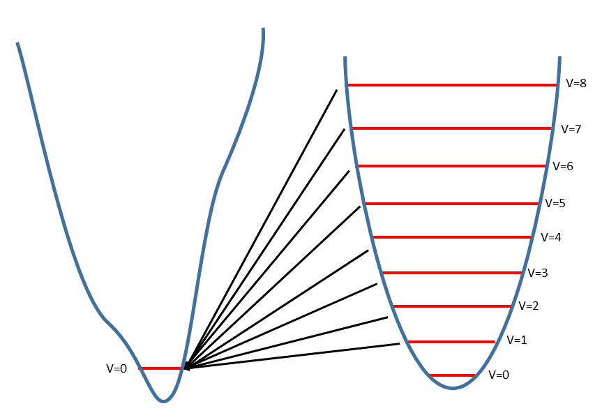
That is to say, on switching on \(\hat{H}^1\) changes the wavefunctions:
\[ \underbrace{ | n^o \rangle }_{\text{unperturbed}} \Rightarrow \underbrace{|n \rangle }_{\text{Perturbed}}\label{7.4.3}\]
and energies (Figure \(\PageIndex{1}\)):
\[ \underbrace{ E_n^o }_{\text{unperturbed}} \Rightarrow \underbrace{E_n }_{\text{Perturbed}} \label{7.4.4}\]
The basic assumption in perturbation theory is that \(H^1\) is sufficiently small that the leading corrections are the same order of magnitude as \(H^1\) itself, and the true energies can be better and better approximated by a successive series of corrections, each of order \(H^1/H^o\) compared with the previous one.
The strategy is to expand the true wavefunction and corresponding eigenenergy as series in \(\hat{H}^1/\hat{H}^o\). These series are then fed into Equation \(\ref{7.4.2}\), and terms of the same order of magnitude in \(\hat{H}^1/\hat{H}^o\) on the two sides are set equal. The equations thus generated are solved one by one to give progressively more accurate results.
To make it easier to identify terms of the same order in \(\hat{H}^1/\hat{H}^o\) on the two sides of the equation, it is convenient to introduce a dimensionless parameter \(\lambda\) which always goes with \(\hat{H}^1\), and then expand both eigenstates and eigenenergies as power series in \(\lambda\),
\[ \begin{align} | n \rangle &= \sum _ i^m \lambda ^i| n^i \rangle \label{7.4.5} \\[4pt] E_n &= \sum_{i=0}^m \lambda ^i E_n^i \label{7.4.6} \end{align}\]
where \(m\) is how many terms in the expansion we are considering. The ket \(|n^i \rangle\) is multiplied by \(\lambda^i\) and is therefore of order \((H^1/H^o)^i\).
\(\lambda\) is purely a bookkeeping device: we will set it equal to 1 when we are through! It’s just there to keep track of the orders of magnitudes of the various terms.
For example, in first order perturbation theory, Equations \(\ref{7.4.5}\) are truncated at \(m=1\) (and setting \(\lambda=1\)):
\[ \begin{align} | n \rangle &\approx | n^o \rangle + | n^1 \rangle \label{7.4.7} \\[4pt] E_n &\approx E_n^o + E_n^1 \label{7.4.8} \end{align}\]
However, let's consider the general case for now. Adding the full expansions for the eigenstate (Equation \(\ref{7.4.5}\)) and energies (Equation \(\ref{7.4.6}\)) into the Schrödinger equation for the perturbation Equation \(\ref{7.4.2}\) in
\[ ( \hat{H}^o + \lambda \hat{H}^1) | n \rangle = E_n| n \rangle \label{7.4.9}\]
we have
\[ (\hat{H}^o + \lambda \hat{H}^1) \left( \sum _ {i=0}^m \lambda ^i| n^i \rangle \right) = \left( \sum_{i=0}^m \lambda^i E_n^i \right) \left( \sum _ {i=0}^m \lambda ^i| n^i \rangle \right) \label{7.4.10}\]
We’re now ready to match the two sides term by term in powers of \(\lambda\). Note that the zeroth-order term, of course, just gives back the unperturbed Schrödinger Equation (Equation \(\ref{7.4.1}\)).
Let's look at Equation \(\ref{7.4.10}\) with the first few terms of the expansion:
\[ \begin{align} (\hat{H}^o + \lambda \hat{H}^1) \left( | n ^o \rangle + \lambda | n^1 \rangle \right) &= \left( E _n^0 + \lambda E_n^1 \right) \left( | n ^o \rangle + \lambda | n^1 \rangle \right) \label{7.4.11} \\[4pt] \hat{H}^o | n ^o \rangle + \lambda \hat{H}^1 | n ^o \rangle + \lambda H^o | n^1 \rangle + \lambda^2 \hat{H}^1| n^1 \rangle &= E _n^0 | n ^o \rangle + \lambda E_n^1 | n ^o \rangle + \lambda E _n^0 | n ^1 \rangle + \lambda^2 E_n^1 | n^1 \rangle \label{7.4.11A} \end{align}\]
Collecting terms in order of \(\lambda\) and coloring to indicate different orders
\[ \underset{\text{zero order}}{\hat{H}^o | n ^o \rangle} + \color{red} \underset{\text{1st order}}{\lambda ( \hat{H}^1 | n ^o \rangle + \hat{H}^o | n^1 \rangle )} + \color{blue} \underset{\text{2nd order}} {\lambda^2 \hat{H}^1| n^1 \rangle} =\color{black}\underset{\text{zero order}}{E _n^0 | n ^o \rangle} + \color{red} \underset{\text{1st order}}{ \lambda (E_n^1 | n ^o \rangle + E _n^0 | n ^1 \rangle )} +\color{blue}\underset{\text{2nd order}}{\lambda^2 E_n^1 | n^1 \rangle} \label{7.4.12}\]
If we expanded Equation \(\ref{7.4.10}\) further we could express the energies and wavefunctions in higher order components.
Zero-Order Terms (\(\lambda=0\))
Collecting the zero order terms in the expansion (black terms in Equation \(\ref{7.4.10}\)) results in just the Schrödinger Equation for the unperturbed system
\[ \hat{H}^o | n^o \rangle = E_n^o | n^o \rangle \label{Zero}\]
First-Order Expression of Energy (\(\lambda=1\))
The summations in Equations \(\ref{7.4.5}\), \(\ref{7.4.6}\), and \(\ref{7.4.10}\) can be truncated at any order of \(\lambda\). For example, the first order perturbation theory has the truncation at \(\lambda=1\). Matching the terms that linear in \(\lambda\) (red terms in Equation \(\ref{7.4.12}\)) and setting \(\lambda=1\) on both sides of Equation \(\ref{7.4.12}\):
\[ \hat{H}^o | n^1 \rangle + \hat{H}^1 | n^o \rangle = E_n^o | n^1 \rangle + E_n^1 | n^o \rangle \label{7.4.13}\]
Equation \(\ref{7.4.13}\) is the key to finding the first-order change in energy \(E_n^1\). Taking the inner product of both sides with \(\langle n^o | \):
\[ \langle n^o | \hat{H}^o | n^1 \rangle + \langle n^o | \hat{H}^1 | n^o \rangle = \langle n^o | E_n^o| n^1 \rangle + \langle n^o | E_n^1 | n^o \rangle \label{7.4.14}\]
since operating the zero-order Hamiltonian on the bra wavefunction (this is just the Schrödinger equation; Equation \(\ref{Zero}\)) is
\[ \langle n^o | \hat{H}^o = \langle n^o | E_n^o \label{7.4.15}\]
and via the orthonormality of the unperturbed \(| n^o \rangle\) wavefunctions both
\[ \langle n^o | n^o \rangle = 1 \label{7.4.16}\]
and Equation \(\ref{7.4.8}\) can be simplified
\[ \bcancel{E_n^o \langle n^o | n^1 \rangle} + \langle n^o | H^1 | n^o \rangle = \bcancel{ E_n^o \langle n^o | n^1 \rangle} + E_n^1 \cancelto{1}{\langle n^o | n^o} \rangle \label{7.4.14new}\]
since the unperturbed set of eigenstates are orthogonal (Equation \ref{7.4.16}) and we can cancel the other term on each side of the equation, we find that
\[ E_n^1 = \langle n^o | \hat{H}^1 | n^o \rangle \label{7.4.17}\]
The first-order change in the energy of a state resulting from adding a perturbing term \(\hat{H}^1\) to the Hamiltonian is just the expectation value of \(\hat{H}^1\) in the unperturbed wavefunctions.
That is, the first order energies (Equation \ref{7.4.13}) are given by
\[ \begin{align} E_n &\approx E_n^o + E_n^1 \\[4pt] &\approx \underbrace{ E_n^o + \langle n^o | H^1 | n^o \rangle}_{\text{First Order Perturbation}} \label{7.4.17.2} \end{align}\]
Estimate the energy of the ground-state and first excited-state wavefunction within first-order perturbation theory of a system with the following potential energy
\[V(x)=\begin{cases}
V_o & 0\leq x\leq L \\
\infty & x< 0 \;\text{and} \; x> L \end{cases} \nonumber\]
Solution
The first step in any perturbation problem is to write the Hamiltonian in terms of a unperturbed component that the solutions (both eigenstates and energy) are known and a perturbation component (Equation \(\ref{7.4.2}\)). For this system, the unperturbed Hamilonian and solutions is the particle in an infiinitely high box and the perturbation is a shift of the potential within the box by \(V_o\).
\[ \hat{H}^1 = V_o \nonumber\]
Using Equation \(\ref{7.4.17}\) for the first-order term in the energy of the ground-state
\[ E_n^1 = \langle n^o | H^1 | n^o \rangle \nonumber\]
with the wavefunctions known from the particle in the box problem
\[ | n^o \rangle = \sqrt{\dfrac{2}{L}} \sin \left ( \dfrac {n \pi}{L} x \right) \nonumber\]
At this stage we can do two problems independently (i.e., the ground-state with \(| 1 \rangle\) and the first excited-state \(| 2 \rangle\)). However, in this case, the first-order perturbation to any particle-in-the-box state can be easily derived.
\[ E_n^1 = \int_0^L \sqrt{\dfrac{2}{L}} \sin \left ( \dfrac {n \pi}{L} x \right) V_o \sqrt{\dfrac{2}{L}} \sin \left ( \dfrac {n \pi}{L} x \right) dx \nonumber\]
or better yet, instead of evaluating this integrals we can simplify the expression
\[ E_n^1 = \langle n^o | H^1 | n^o \rangle = \langle n^o | V_o | n^o \rangle = V_o \langle n^o | n^o \rangle = V_o \nonumber\]
so via Equation \(\ref{7.4.17.2}\), the energy of each perturbed eigenstate is
\[ \begin{align*} E_n &\approx E_n^o + E_n^1 \\[4pt] &\approx \dfrac{h^2}{8mL^2}n^2 + V_o \end{align*}\]
While this is the first order perturbation to the energy, it is also the exact value.
Estimate the energy of the ground-state wavefunction within first-order perturbation theory of a system with the following potential energy
\[V(x)=\begin{cases}
V_o & 0\leq x\leq L/2 \\
\infty & x< 0 \; and\; x> L \end{cases} \nonumber\]
Solution
As with Example \(\PageIndex{1}\), we recognize that unperturbed component of the problem (Equation \(\ref{7.4.2}\)) is the particle in an infinitely high well. For this system, the unperturbed Hamiltonian and solution is the particle in an infinitely high box and the perturbation is a shift of the potential within half a box by \(V_o\). This is essentially a step function.
Using Equation \(\ref{7.4.17}\) for the first-order term in the energy of the any state
\[ \begin{align*} E_n^1 &= \langle n^o | H^1 | n^o \rangle \\[4pt] &= \int_0^{L/2} \sqrt{\dfrac{2}{L}} \sin \left ( \dfrac {n \pi}{L} x \right) V_o \sqrt{\dfrac{2}{L}} \sin \left ( \dfrac {n \pi}{L} x \right) dx + \int_{L/2}^L \sqrt{\dfrac{2}{L}} \sin \left ( \dfrac {n \pi}{L} x \right) 0 \sqrt{\dfrac{2}{L}} \sin \left ( \dfrac {n \pi}{L} x \right) dx \end{align*}\]
The second integral is zero and the first integral is simplified to
\[ E_n^1 = \dfrac{2}{L} \int_0^{L/2} V_o \sin^2 \left( \dfrac {n \pi}{L} x \right) dx \nonumber\]
this is evaluated to
\[ \begin{align*} E_n^1 &= \dfrac{2V_o}{L} \left[ \dfrac{-1}{2 \dfrac{\pi n}{a}} \cos \left( \dfrac {n \pi}{L} x \right) \sin \left( \dfrac {n \pi}{L} x \right) + \dfrac{x}{2} \right]_0^{L/2} \\[4pt] &= \dfrac{2V_o}{\cancel{L}} \dfrac{\cancel{L}}{4} = \dfrac{V_o}{2} \end{align*}\]
The energy of each perturbed eigenstate, via Equation \(\ref{7.4.17.2}\), is
\[ \begin{align*} E_n &\approx E_n^o + \dfrac{V_o}{2} \\[4pt] &\approx \dfrac{h^2}{8mL^2}n^2 + \dfrac{V_o}{2} \end{align*}\]
First-Order Expression of Wavefunction (\(\lambda=1\))
The general expression for the first-order change in the wavefunction is found by taking the inner product of the first-order expansion (Equation \(\ref{7.4.13}\)) with the bra \( \langle m^o |\) with \(m \neq n\),
\[ \langle m^o | H^o | n^1 \rangle + \langle m^o |H^1 | n^o \rangle = \langle m^o | E_n^o | n^1 \rangle + \langle m^o |E_n^1 | n^o \rangle \label{7.4.18}\]
Last term on right side of Equation \(\ref{7.4.18}\)
The last integral on the right hand side of Equation \(\ref{7.4.18}\) is zero, since \(m \neq n\) so
\[ \langle m^o |E_n^1 | n^o \rangle = E_n^1 \langle m^o | n^o \rangle \label{7.4.19}\]
and
\[\langle m^o | n^0 \rangle = 0 \label{7.4.20}\]
First term on right side of Equation \(\ref{7.4.18}\)
The first integral is more complicated and can be expanded back into the \(H^o\)
\[ E_m^o \langle m^o | n^1 \rangle = \langle m^o|E_m^o | n^1 \rangle = \langle m^o | H^o | n^1 \rangle \label{7.4.21}\]
since
\[ \langle m^o | H^o = \langle m^o | E_m^o \label{7.4.22}\]
so
\[ \langle m^o | n^1 \rangle = \dfrac{\langle m^o | H^1 | n^o \rangle}{ E_n^o - E_m^o} \label{7.4.23}\]
and therefore the wavefunction corrected to first order is:
\[ \begin{align} | n \rangle &\approx | n^o \rangle + | n^1 \rangle \\[4pt] &\approx \underbrace{| n^o \rangle + \sum _{m \neq n} \dfrac{|m^o \rangle \langle m^o | H^1| n^o \rangle }{E_n^o - E_m^o}}_{\text{First Order Perturbation Theory}} \label{7.4.24} \end{align}\]
Equation \(\ref{7.4.24}\) is essentially is an expansion of the unknown wavefunction correction as a linear combination of known unperturbed wavefunctions \(\ref{7.4.24.2}\):
\[ \begin{align} | n \rangle &\approx | n^o \rangle + | n^1 \rangle \\[4pt] &\approx | n^o \rangle + \sum _{m \neq n} c_{m,n} |m^o \rangle \label{7.4.24.2} \end{align}\]
with the expansion coefficients determined by
\[ c_{m,n} = \dfrac{\langle m^o | H^1| n^o \rangle }{E_n^o - E_m^o} \label{7.4.24.3}\]
This is justified since the set of original zero-order wavefunctions forms a complete basis set that can describe any function.
Calculating the first order perturbation to the wavefunctions is in general an infinite sum of off diagonal matrix elements of \(H^1\) (Figure \(\PageIndex{2}\)).
- However, the denominator argues that terms in this sum will be weighted by states that are of comparable energy. That means in principle, these sum can be truncated easily based off of some criterion.
- Another point to consider is that many of these matrix elements will equal zero depending on the symmetry of the \(\{| n^o \rangle \}\) basis and \(H^1\) (e.g., some \(\langle m^o | H^1| n^o \rangle\) integrals in Equation \(\ref{7.4.24}\) could be zero due to the integrand having an odd symmetry; see Example \(\PageIndex{3}\)).
The denominators in Equation \(\ref{7.4.24}\) argues that terms in this sum will be preferentially dictated by states that are of comparable energy. That is, eigenstates that have energies significantly greater or lower than the unperturbed eigenstate will weakly contribute to the perturbed wavefunction.
Estimate the energy of the ground-state wavefunction associated with the Hamiltonian using perturbation theory
\[ \hat{H} = \dfrac{-\hbar}{2m} \dfrac{d^2}{dx^2} + \dfrac{1}{2} kx^2 + \epsilon x^3 \nonumber\]
Solution
The first step in a perturbation theory problem is to identify the reference system with the known eigenstates and energies. For this example, this is clearly the harmonic oscillator model.
Energy
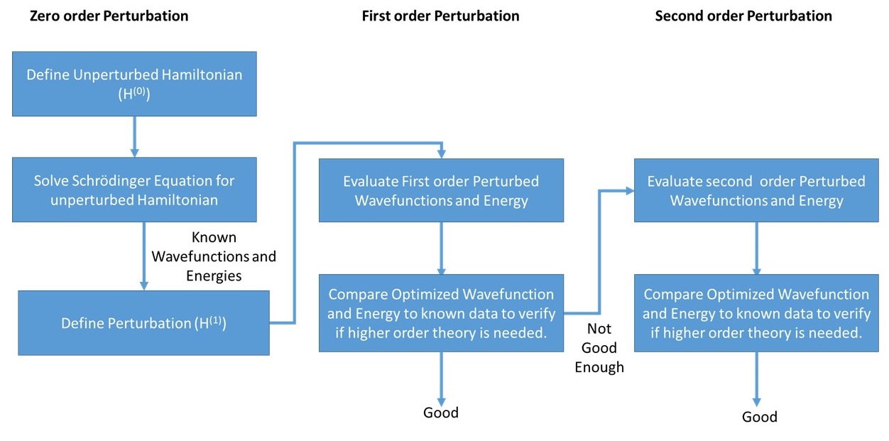
The first steps in flowchart for applying perturbation theory (Figure \(\PageIndex{1}\)) is to separate the Hamiltonian of the difficult (or unsolvable) problem into a solvable one with a perturbation. For this case, we can rewrite the Hamiltonian as
\[ \hat{H}^{o} + \hat{H}^{1} \nonumber\]
where
- \(\hat{H}^{o}\) is the Hamitonian for the standard Harmonic Oscillator with known eigenstates and eigenenergies \[ \hat{H}^{(0)}= \dfrac{-\hbar}{2m} \dfrac{d^2}{dx^2} + \dfrac{1}{2} kx^2 \nonumber\]
- \(\hat{H}^{1}\) is the pertubtiation \[\hat{H}^{1} = \epsilon x^3 \nonumber\]
The first order perturbation is given by Equation \(\ref{7.4.17}\), which for this problem is
\[E_n^1 = \langle n^o | \epsilon x^3 | n^o \rangle \nonumber\]
Notice that the integrand has an odd symmetry (i.e., \(f(x)=-f(-x)\)) with the perturbation Hamiltonian being odd and the ground state harmonic oscillator wavefunctions being even. So
\[E_n^1=0 \nonumber\]
This means to first order pertubation theory, this cubic terms does not alter the ground state energy (via Equation \(\ref{7.4.17.2})\). However, this is not the case if second-order perturbation theory were used, which is more accurate (not shown).
Wavefunction
Calculating the first order perturbation to the wavefunctions (Equation \(\ref{7.4.24}\)) is more difficult than energy since multiple integrals must be evaluated (an infinite number if symmetry arguments are not applicable). The harmonic oscillator wavefunctions are often written in terms of \(Q\), the unscaled displacement coordinate:
\[ | \Psi _v (x) \rangle = N_v'' H_v (\sqrt{\alpha} Q) e^{-\alpha Q^2/ 2} \nonumber \]
with \(\alpha\)
\[ \alpha =1/\sqrt{\beta} = \sqrt{\dfrac{k \mu}{\hbar ^2}} \nonumber\]
and
\[ N_v'' = \sqrt {\dfrac {1}{2^v v!}} \left(\dfrac{\alpha}{\pi}\right)^{1/4} \nonumber\]
Let's consider only the first six wavefunctions that use these Hermite polynomials \(H_v (x)\):
- \(H_0 = 1\)
- \(H_1 = 2x\)
- \(H_2 = -2 + 4x^2\)
- \(H_3 = -12x + 8x^3\)
- \(H_4 = 12 - 48x^2 +16x^4\)
- \(H_5 = 120x - 160x^3 + 32x^5\)
The first order perturbation to the ground-state wavefunction (Equation \(\ref{7.4.24}\))
\[ | 0^1 \rangle = \sum _{m \neq 0}^5 \dfrac{|m^o \rangle \langle m^o | H^1| 0^o \rangle }{E_0^o - E_m^o} \label{energy1}\]
given these truncated wavefunctions (we should technically use the infinite sum) and that we are considering only the ground state with \(n=0\):
\[| 0^1 \rangle = \dfrac{ \langle 1^o | H^1| 0^o \rangle }{E_0^o - E_1^o} |1^o \rangle + \dfrac{ \langle 2^o | H^1| 0^o \rangle }{E_0^o - E_2^o} |2^o \rangle + \dfrac{ \langle 3^o | H^1| 0^o \rangle }{E_0^o - E_3^o} |3^o \rangle + \dfrac{ \langle 4^o | H^1| 0^o \rangle }{E_0^o - E_4^o} |4^o \rangle + \dfrac{ \langle 5^o | H^1| 0^o \rangle }{E_0^o - E_5^o} |5^o \rangle \nonumber\]
We can use symmetry of the perturbation and unperturbed wavefunctions to solve the integrals above. We know that the unperturbed harmonic oscillator wavefunctions \(\{|n^{0}\} \rangle\) alternate between even (when \(v\) is even) and odd (when \(v\) is odd) as shown previously. Since the perturbation is an odd function, only when \(m= 2k+1\) with \(k=1,2,3\) would these integrals be non-zero (i.e., for \(m=1,3,5, ...\)).
So of the original five unperturbed wavefunctions, only \(|m=1\rangle\), \(|m=3\rangle\), and \(|m=5 \rangle\) mix to make the first-order perturbed ground-state wavefunction so
\[| 0^1 \rangle = \dfrac{ \langle 1^o | H^1| 0^o \rangle }{E_0^o - E_1^o} |1^o \rangle + \dfrac{ \langle 3^o | H^1| 0^o \rangle }{E_0^o - E_3^o} |3^o \rangle + \dfrac{ \langle 5^o | H^1| 0^o \rangle }{E_0^o - E_5^o} |5^o \rangle \nonumber\]
At this stage, the integrals have to be manually calculated using the defined wavefuctions above, which is left as an exercise. Notice that each unperturbed wavefunction that can "mix" to generate the perturbed wavefunction will have a reciprocally decreasing contribution (w.r.t. energy) due to the growing denominator in Equation \ref{energy1}.
Use perturbation theory to estimate the energy of the ground-state wavefunction associated with this Hamiltonian
\[ \hat{H} = \dfrac{-\hbar}{2m} \dfrac{d^2}{dx^2} + \dfrac{1}{2} kx^2 + \gamma x^4 \nonumber.\]
- Answer
-
The model that we are using is the harmonic oscillator model which has a Hamiltonian
\[H^{0}=-\frac{\hbar}{2 m} \frac{d^2}{dx^2}+\dfrac{1}{2} k x^2 \nonumber\]
Making the perturbed Hamiltonian
\[H^{1}=\gamma x^{4} \nonumber\]
To find the perturbed energy we approximate it using Equation \ref{7.4.17.2}
\[E^{1}= \langle n^{0}\left|H^{1}\right| n^{0} \rangle \nonumber\]
where is the wavefunction of the ground state harmonic oscillator
\[n^{0}=\left(\frac{a}{\pi}\right)^{\left(\frac{1}{4}\right)} e^{-\frac{ax^2}{2}} \nonumber\]
When we substitute in the Hamiltonian and the wavefunction we get
\[E^{1}=\left\langle\left(\frac{a}{\pi}\right)^{\left(\frac{1}{4}\right)} e^{-\frac{ax^2}{2}}\right|\gamma x^{4}\left|\left(\frac{a}{\pi}\right)^{\left(\frac{1}{4}\right)} e^{-\frac{ax^2}{2}} \right \rangle \nonumber\]
Changing this into integral form, and combining the wavefunctions,
\[\begin{align*} E^{1} &=\int_{-\infty}^{\infty}\left(\frac{a}{\pi}\right)^{\left(\frac{1}{2}\right)} e^{\frac{-ax^2}{2}} \gamma x^{4} dx \\[4pt] &=\gamma\left(\frac{a}{\pi}\right)^{\frac{1}{2}} \int_{-\infty}^{\infty} x^{4} e^{-a x^2} d x \end{align*} \]
Now we use the integral table value
\[\int_{0}^{\infty} x^{2 \pi} e^{-a x^2} dx=\frac{1 \cdot 3 \cdot 5 \ldots (2 n-1)}{2^{m+1} a^{n}}\left(\frac{\pi}{a}\right)^{\frac{1}{2}} \nonumber\]
Where we plug in \(\mathrm{n}=2\) and \(\mathrm{a}=\alpha\) for our integral
\[\begin{aligned}E^{1} &=2 \gamma\left(\frac{a}{\pi}\right)^{\left(\frac{1}{2}\right)} \int_{0}^{\infty} x^{4} e^{-a x^2} d x \\
E^{1} &=2 \gamma\left(\frac{a}{\pi}\right)^{\left(\frac{1}{2}\right)} \frac{1\cdot 3}{2^{3} a^2}\left(\frac{\pi}{a}\right)^{\frac{1}{2}}\end{aligned} \nonumber\]This is our perturbed energy
Now we have to find our ground state energy using the formula for the energy of a harmonic oscillator that we already know,
\[E_{r}^{0}=\left(v+\dfrac{1}{2}\right) hv \nonumber\]
Where in the ground state \(v=0\) so the energy for the ground state of the quantum harmonic oscillator is
\[E_{\mathrm{r}}^{0}=\frac{1}{2} h v \nonumber\]
Putting both of our energy terms together gives us the ground state energy of the wavefunction of the given Hamiltonian,
\[
\begin{array}{c}
{E=E^{0}+E^{1}} \\
{E=\frac{1}{2} h v+\gamma \frac{3}{4 a^2}}
\end{array}
\nonumber \]
Second-Order Terms (\(\lambda=2\))
There are higher energy terms in the expansion of Equation \(\ref{7.4.5}\) (e.g., the blue terms in Equation \(\ref{7.4.12}\)), but are not discussed further here other than noting the whole perturbation process is an infinite series of corrections that ideally converge to the correct answer. It is truncating this series as a finite number of steps that is the approximation. The general approach to perturbation theory applications is giving in the flowchart in Figure \(\PageIndex{1}\).
It should be noted that there are problems that cannot be solved using perturbation theory, even when the perturbation is very weak, although such problems are the exception rather than the rule. One such case is the one-dimensional problem of free particles perturbed by a localized potential of strength \(\lambda\). Switching on an arbitrarily weak attractive potential causes the \(k=0\) free particle wavefunction to drop below the continuum of plane wave energies and become a localized bound state with binding energy of order \(\lambda^2\). However, changing the sign of \(\lambda\) to give a repulsive potential there is no bound state, the lowest energy plane wave state stays at energy zero. Therefore the energy shift on switching on the perturbation cannot be represented as a power series in \(\lambda\), the strength of the perturbation.
Contributors
Michael Fowler (Beams Professor, Department of Physics, University of Virginia)
http://fizika.unios.hr/~ilukacevic/d...ion_theory.pdf