
7.2: Linear Variational Method and the Secular Determinant
- Page ID
- 210833

\( \newcommand{\vecs}[1]{\overset { \scriptstyle \rightharpoonup} {\mathbf{#1}} } \)
\( \newcommand{\vecd}[1]{\overset{-\!-\!\rightharpoonup}{\vphantom{a}\smash {#1}}} \)
\( \newcommand{\id}{\mathrm{id}}\) \( \newcommand{\Span}{\mathrm{span}}\)
( \newcommand{\kernel}{\mathrm{null}\,}\) \( \newcommand{\range}{\mathrm{range}\,}\)
\( \newcommand{\RealPart}{\mathrm{Re}}\) \( \newcommand{\ImaginaryPart}{\mathrm{Im}}\)
\( \newcommand{\Argument}{\mathrm{Arg}}\) \( \newcommand{\norm}[1]{\| #1 \|}\)
\( \newcommand{\inner}[2]{\langle #1, #2 \rangle}\)
\( \newcommand{\Span}{\mathrm{span}}\)
\( \newcommand{\id}{\mathrm{id}}\)
\( \newcommand{\Span}{\mathrm{span}}\)
\( \newcommand{\kernel}{\mathrm{null}\,}\)
\( \newcommand{\range}{\mathrm{range}\,}\)
\( \newcommand{\RealPart}{\mathrm{Re}}\)
\( \newcommand{\ImaginaryPart}{\mathrm{Im}}\)
\( \newcommand{\Argument}{\mathrm{Arg}}\)
\( \newcommand{\norm}[1]{\| #1 \|}\)
\( \newcommand{\inner}[2]{\langle #1, #2 \rangle}\)
\( \newcommand{\Span}{\mathrm{span}}\) \( \newcommand{\AA}{\unicode[.8,0]{x212B}}\)
\( \newcommand{\vectorA}[1]{\vec{#1}} % arrow\)
\( \newcommand{\vectorAt}[1]{\vec{\text{#1}}} % arrow\)
\( \newcommand{\vectorB}[1]{\overset { \scriptstyle \rightharpoonup} {\mathbf{#1}} } \)
\( \newcommand{\vectorC}[1]{\textbf{#1}} \)
\( \newcommand{\vectorD}[1]{\overrightarrow{#1}} \)
\( \newcommand{\vectorDt}[1]{\overrightarrow{\text{#1}}} \)
\( \newcommand{\vectE}[1]{\overset{-\!-\!\rightharpoonup}{\vphantom{a}\smash{\mathbf {#1}}}} \)
\( \newcommand{\vecs}[1]{\overset { \scriptstyle \rightharpoonup} {\mathbf{#1}} } \)
\( \newcommand{\vecd}[1]{\overset{-\!-\!\rightharpoonup}{\vphantom{a}\smash {#1}}} \)
\(\newcommand{\avec}{\mathbf a}\) \(\newcommand{\bvec}{\mathbf b}\) \(\newcommand{\cvec}{\mathbf c}\) \(\newcommand{\dvec}{\mathbf d}\) \(\newcommand{\dtil}{\widetilde{\mathbf d}}\) \(\newcommand{\evec}{\mathbf e}\) \(\newcommand{\fvec}{\mathbf f}\) \(\newcommand{\nvec}{\mathbf n}\) \(\newcommand{\pvec}{\mathbf p}\) \(\newcommand{\qvec}{\mathbf q}\) \(\newcommand{\svec}{\mathbf s}\) \(\newcommand{\tvec}{\mathbf t}\) \(\newcommand{\uvec}{\mathbf u}\) \(\newcommand{\vvec}{\mathbf v}\) \(\newcommand{\wvec}{\mathbf w}\) \(\newcommand{\xvec}{\mathbf x}\) \(\newcommand{\yvec}{\mathbf y}\) \(\newcommand{\zvec}{\mathbf z}\) \(\newcommand{\rvec}{\mathbf r}\) \(\newcommand{\mvec}{\mathbf m}\) \(\newcommand{\zerovec}{\mathbf 0}\) \(\newcommand{\onevec}{\mathbf 1}\) \(\newcommand{\real}{\mathbb R}\) \(\newcommand{\twovec}[2]{\left[\begin{array}{r}#1 \\ #2 \end{array}\right]}\) \(\newcommand{\ctwovec}[2]{\left[\begin{array}{c}#1 \\ #2 \end{array}\right]}\) \(\newcommand{\threevec}[3]{\left[\begin{array}{r}#1 \\ #2 \\ #3 \end{array}\right]}\) \(\newcommand{\cthreevec}[3]{\left[\begin{array}{c}#1 \\ #2 \\ #3 \end{array}\right]}\) \(\newcommand{\fourvec}[4]{\left[\begin{array}{r}#1 \\ #2 \\ #3 \\ #4 \end{array}\right]}\) \(\newcommand{\cfourvec}[4]{\left[\begin{array}{c}#1 \\ #2 \\ #3 \\ #4 \end{array}\right]}\) \(\newcommand{\fivevec}[5]{\left[\begin{array}{r}#1 \\ #2 \\ #3 \\ #4 \\ #5 \\ \end{array}\right]}\) \(\newcommand{\cfivevec}[5]{\left[\begin{array}{c}#1 \\ #2 \\ #3 \\ #4 \\ #5 \\ \end{array}\right]}\) \(\newcommand{\mattwo}[4]{\left[\begin{array}{rr}#1 \amp #2 \\ #3 \amp #4 \\ \end{array}\right]}\) \(\newcommand{\laspan}[1]{\text{Span}\{#1\}}\) \(\newcommand{\bcal}{\cal B}\) \(\newcommand{\ccal}{\cal C}\) \(\newcommand{\scal}{\cal S}\) \(\newcommand{\wcal}{\cal W}\) \(\newcommand{\ecal}{\cal E}\) \(\newcommand{\coords}[2]{\left\{#1\right\}_{#2}}\) \(\newcommand{\gray}[1]{\color{gray}{#1}}\) \(\newcommand{\lgray}[1]{\color{lightgray}{#1}}\) \(\newcommand{\rank}{\operatorname{rank}}\) \(\newcommand{\row}{\text{Row}}\) \(\newcommand{\col}{\text{Col}}\) \(\renewcommand{\row}{\text{Row}}\) \(\newcommand{\nul}{\text{Nul}}\) \(\newcommand{\var}{\text{Var}}\) \(\newcommand{\corr}{\text{corr}}\) \(\newcommand{\len}[1]{\left|#1\right|}\) \(\newcommand{\bbar}{\overline{\bvec}}\) \(\newcommand{\bhat}{\widehat{\bvec}}\) \(\newcommand{\bperp}{\bvec^\perp}\) \(\newcommand{\xhat}{\widehat{\xvec}}\) \(\newcommand{\vhat}{\widehat{\vvec}}\) \(\newcommand{\uhat}{\widehat{\uvec}}\) \(\newcommand{\what}{\widehat{\wvec}}\) \(\newcommand{\Sighat}{\widehat{\Sigma}}\) \(\newcommand{\lt}{<}\) \(\newcommand{\gt}{>}\) \(\newcommand{\amp}{&}\) \(\definecolor{fillinmathshade}{gray}{0.9}\)- Understand how the variational method can be expanded to include trial wavefunctions that are a linear combination of functions with coefficients that are the parameters to be varied.
- To be able to construct secular equations to solve the minimization procedure intrinsic to the variational method approach.
- To map the secular equations into the secular determinant
- To understand how the Linear Combination of Atomic Orbital (LCAO) approximation is a specific application of the linear variational method.
A special type of variation widely used in the study of molecules is the so-called linear variation function, where the trial wavefunction is a linear combination of \(N\) linearly independent functions (often atomic orbitals) that not the eigenvalues of the Hamiltonian (since they are not known). For example
\[| \psi_{trial} \rangle = \sum_{j=1}^N a_j |\phi_j \rangle \label{Ex1}\]
and
\[ \langle \psi_{trial} | = \sum_{j=1}^N a_j^* \langle \phi_j | \label{Ex2}\]
In these cases, one says that a 'linear variational' calculation is being performed.
The set of functions {\(\phi_j\)} are called the 'linear variational' basis functions and are nothing more than members of a set of functions that are convenient to deal with. However, they are typically not arbitrary and are usually selected to address specific properties of the system:
- to obey all of the boundary conditions that the exact state \(| \psi _{trial} \rangle\) obeys,
- to be functions of the the same coordinates as \(| \psi _{trial} \rangle\),
- to be of the same symmetry as \(| \psi _{trial} \rangle\), and
- to be convenient to evaluate Hamiltonian terms elements \(\langle \phi_i|H|\phi_j \rangle\).
Beyond these conditions, nothing other than effort can limit the selection and number of such basis functions in the expansions in Equations \(\ref{Ex1}\) and \(\ref{Ex2}\).
As discussed in Section 7.1, the variational energy for a generalized trial wavefunction is
\[ E_{trial} = \dfrac{ \langle \psi _{trial}| \hat {H} | \psi _{trial} \rangle}{\langle \psi _{trial} | \psi _{trial} \rangle} \label{7.1.8}\]
Substituting Equations \ref{Ex1} and \ref{Ex2} into Equation \ref{7.1.8} involves addressing the numerator and denominator individually. For the numerator, the integral can be expanded thusly:
\[\begin{align} \langle\psi_{trial} |H| \psi_{trial} \rangle &= \sum_{i}^{N} \sum_{j} ^{N}a_i^{*} a_j \langle \phi_i|H|\phi_j \rangle. \\[4pt] &= \sum_{i,\,j} ^{N,\,N}a_i^{*} a_j \langle \phi_i|H|\phi_j \rangle. \label{MatrixElement}\end{align}\]
We can rewrite the following integral in Equation \ref{MatrixElement} as a function of the basis elements (not the trial wavefunction) as
\[ H_{ij} = \langle \phi_i|H|\phi_j \rangle\]
So the numerator of the right side of Equation \ref{7.1.8} becomes
\[\langle\psi_{trial} |H| \psi_{trial} \rangle = \sum_{i,\,j} ^{N,\,N}a_i^{*} a_j H_{ij} \label{numerator}\]
Similarly, the denominator of the right side of Equation \ref{7.1.8} can be expanded
\[\langle \psi_{trial}|\psi_{trial} \rangle = \sum_{i,\,j} ^{N,\,N}a_i^{*} a_j \langle \phi_i | \phi_j \rangle \label{overlap}\]
We often simplify the integrals on the right side of Equation \ref{overlap} as
\[ S_{ij} = \langle \phi_i|\phi_j \rangle \]
where \(S_{ij}\) are overlap integrals between the different {\(\phi_j\)} basis functions. Equation \ref{overlap} is thus expressed as
\[\langle \psi_{trial}|\psi_{trial} \rangle = \sum_{i,\,j} ^{N,\,N}a_i^{*} a_j S_{ij} \label{denominator}\]
There is no explicit rule that the {\(\phi_j\)} functions have to be orthogonal or normalized functions, although they often are selected that way for convenience. Therefore, a priori, \(S_{ij}\) does not have to be \(\delta_{ij}\).
Substituting Equations \ref{numerator} and \ref{denominator} into the variational energy formula (Equation \ref{7.1.8}) results in
\[ E_{trial} = \dfrac{ \displaystyle \sum_{i,\,j} ^{N,\,N}a_i^{*} a_j H_{ij} }{ \displaystyle \sum_{i,\,j} ^{N,\,N}a_i^{*} a_j S_{ij} } \label{Var}\]
For such a trial wavefunction as Equation \ref{Ex1}, the variational energy depends quadratically on the 'linear variational' \(a_j\) coefficients. These coefficients can be varied just like the parameters in the trial functions of Section 7.1 to find the optimized trial wavefunction (\(| \psi_{trial} \rangle\)) that approximates the true wavefunction (\(| \psi \rangle\)) that we cannot analytically solve for.
Minimizing the Variational Energy
The expression for variational energy (Equation \ref{Var}) can be rearranged
\[E_{trial} \sum_{i,\,j} ^{N,\,N} a_i^*a_j S_{ij} = \sum_{i,\,j} ^{N,\,N} a_i^* a_j H_{ij} \label{7.2.9}\]
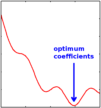
The optimum coefficients are found by searching for minima in the variational energy landscape spanned by varying the \(\{a_i\}\) coefficients (Figure \(\PageIndex{1}\)).
We want to minimize the energy with respect to the linear coefficients \(\{a_i\}\), which requires that
\[\dfrac{\partial E_{trial}}{\partial a_i}= 0\]
for all \(i\).
Differentiating both sides of Equation \(\ref{7.2.9}\) for the \(k^{th}\) coefficient gives,
\[ \dfrac{\partial E_{trial}}{\partial a_k} \sum_{i,\,j} ^{N,\,N} a_i^*a_j S_{ij}+ E_{trial} \sum_i \sum_j \left[ \dfrac{ \partial a_i^*}{\partial a_k} a_j + \dfrac {\partial a_j}{\partial a_k} a_i^* \right ]S_{ij} = \sum_{i,\,j} ^{N,\,N} \left [ \dfrac{\partial a_i^*}{\partial a_k} a_j + \dfrac{ \partial a_j}{\partial a_k}a_i^* \right] H_{ij} \label{7.2.10}\]
Since the coefficients are independent
\[\dfrac{\partial a_i^*}{ \partial a_k} = \delta_{ik}\]
and
\[S_{ij} = S_{ji}\]
and also since the Hamiltonian is a Hermitian Operator (see below)
\[H_{ij} =H_{ji}\]
then Equation \(\ref{7.2.10}\) simplifies to
\[ \dfrac{\partial E_{trial}}{\partial a_k} \sum_i \sum_j a_i^*a_j S_{ij}+ 2E_{trial} \sum_i a_i S_{ik} = 2 \sum_i a_i H_{ik} \label{7.2.11}\]
At the minimum variational energy, when
\[\dfrac{\partial E_{trial}}{\partial a_k} = 0\]
then Equation \(\ref{7.2.11}\) gives
\[ {\sum _i^N a_i (H_{ik}–E_{trial} S_{ik}) = 0} \label{7.2.12}\]
for all \(k\). The equations in \(\ref{7.2.12}\) are call the Secular Equations.
Hermitian operators are operators that satisfy the general formula
\[ \langle \phi_i | \hat{A} | \phi_j \rangle = \langle \phi_j | \hat{A} | \phi_i \rangle \label{Herm1}\]
If that condition is met, then \(\hat{A}\) is a Hermitian operator. For any operator that generates a real eigenvalue (e.g., observables), then that operator is Hermitian. The Hamiltonian \(\hat{H}\) meets the condition and a Hermitian operator. Equation \ref{Herm1} can be rewriten as
\[A_{ij} =A_{ji}^*\]
where
\[A_{ij} = \langle \phi_i | \hat{A} | \phi_j \rangle\]
and
\[A_{ji} = \langle \phi_j | \hat{A} | \phi_i \rangle\]
Therefore, when applied to the Hamiltonian operator
\[H_{ij}^* =H_{ji}.\]
If the functions \(\{|\phi_j\rangle \}\) are orthonormal, then the overlap matrix \(S\) reduces to the unit matrix (one on the diagonal and zero every where else) and the Secular Equations in Equation \ref{7.2.12} reduces to the more familiar Eigenvalue form:
\[ \sum\limits_i^N H_{ij}a_j = E_{trial} a_i .\label{seceq2}\]
Hence, the secular equation, in either form, have as many eigenvalues \(E_i\) and eigenvectors {\(C_{ij}\)} as the dimension of the \(H_{ij}\) matrix as the functions in \(| \psi_{trail} \rangle\) (Example \ref{Ex1}). It can also be shown that between successive pairs of the eigenvalues obtained by solving the secular problem at least one exact eigenvalue must occur (i.e.,\( E_{i+1} > E_{exact} > E_i\), for all i). This observation is referred to as 'the bracketing theorem'.
Variational methods, in particular the linear variational method, are the most widely used approximation techniques in quantum chemistry. To implement such a method one needs to know the Hamiltonian \(H\) whose energy levels are sought and one needs to construct a trial wavefunction in which some 'flexibility' exists (e.g., as in the linear variational method where the \(a_j\) coefficients can be varied). This tool will be used to develop several of the most commonly used and powerful molecular orbital methods in chemistry.
The Secular Determinant
From the secular equations with an orthonormal functions (Equation \ref{seceq2}), we have \(k\) simultaneous secular equations in \(k\) unknowns. These equations can also be written in matrix notation, and for a non-trivial solution (i.e. \(c_i \neq 0\) for all \(i\)), the determinant of the secular matrix must be equal to zero.
\[ { | H_{ik}–ES_{ik}| = 0} \label{7.2.13}\]
- The determinant is a real number, it is not a matrix.
- The determinant can be a negative number.
- It is not associated with absolute value at all except that they both use vertical lines.
- The determinant only exists for square matrices (\(2 \times 2\), \(3 \times 3\), ..., \(n \times n\)). The determinant of a \(1 \times 1\) matrix is that single value in the determinant.
- The inverse of a matrix will exist only if the determinant is not zero.
The determinant can be evaluated using an expansion method involving minors and cofactors. Before we can use them, we need to define them. It is the product of the elements on the main diagonal minus the product of the elements off the main diagonal. In the case of a \(2 \times 2\) matrix, the specific formula for the determinant is
\[{\displaystyle {\begin{aligned}|A|={\begin{vmatrix}a&b\\c&d\end{vmatrix}}=ad-bc.\end{aligned}}}\]
Similarly, suppose we have a \(3 \times 3\) matrix \(A\), and we want the specific formula for its determinant \(|A|\):
\[{\displaystyle {\begin{aligned}|A|={\begin{vmatrix}a&b&c\\d&e&f\\g&h&i\end{vmatrix}}&=a\,{\begin{vmatrix}e&f\\h&i\end{vmatrix}}-b\,{\begin{vmatrix}d&f\\g&i\end{vmatrix}}+c\,{\begin{vmatrix}d&e\\g&h\end{vmatrix}}\\&=aei+bfg+cdh-ceg-bdi-afh.\end{aligned}}}\]
To solve Equation \ref{7.2.13}, the determinate should be expanded and then set to zero. That generates a polynomial (called a characteristic equation) that can be directly solved with linear algebra methods or numerically.
If \(|\psi_{trial} \rangle\) is a linear combination of two functions. In math terms,
\[|\psi_{trial} \rangle= \sum_{n=1}^{N=2} a_n |f_n\rangle = a_1 |\phi_1 \rangle + a_2 | \phi_2 \rangle \nonumber \]
then the secular determinant (Equation \(\ref{7.2.13}\)), in matrix formulation would look like this
\[\begin{vmatrix} H_{11}-E_{trial}S_{11}&H_{12}-E_{trial}S_{12} \\ H_{12}-E_{trial}S_{12}&H_{22}-E_{trial}S_{22}\end{vmatrix}=0 \nonumber\]
Solution
Solving the secular equations is done by finding \(E_{trial}\) and putting the value into the expansion of the secular determinant
\[a_1^2 H_{11} + 2a_1 a_2 H_{12}+ a_2^2 H_{22}=0 \nonumber\]
and
\[a_1(H_{12} - E_{trial}S_{12}) + a_2(H_{22} - E_{trial}S_{22}) = 0 \nonumber\]
Equation \(\ref{7.2.13}\) can be solved to obtain the energies \(E\). When arranged in order of increasing energy, these provide approximations to the energies of the first \(k\) states (each having an energy higher than the true energy of the state by virtue of the variation theorem). To find the energies of a larger number of states we simply use a greater number of basis functions \(\{\phi_i\}\) in the trial wavefunction (Example \ref{Ex1}). To obtain the approximate wavefunction for a particular state, we substitute the appropriate energy into the secular equations and solve for the coefficients \(a_i\).
Using this method it is possible to find all the coefficients \(a_1 \ldots a_k\) in terms of one coefficient; normalizing the wavefunction provides the absolute values for the coefficients.
Trial wavefunctions that consist of linear combinations of simple functions
\[ | \psi(r) \rangle = \sum_i a_i | \phi_i(r) \rangle \nonumber\]
form the basis of the Linear Combination of Atomic Orbitals (LCAO) method introduced by Lennard and Jones and others to compute the energies and wavefunctions of atoms and molecules. The functions \(\{| \phi_i \rangle \}\) are selected so that matrix elements can be evaluated analytically. Two basis sets of atomic orbitals functions can be used: Slater type and Gaussian type:
Slater orbitals using Hydrogen-like wavefunctions
\[ | \phi_i \rangle = Y_{l}^{m}(\theta,\phi) e ^{-\alpha r} \nonumber\]
and Gaussian orbitals of the form
\[ | \phi_i \rangle = Y_{l}^{m}(\theta,\phi) e ^{-\alpha r^2} \nonumber\]
are the most widely used forms, where \(Y_l^m(\theta,\phi)\) are the spherical harmonics that represent the angular part of of the atomic orbitals. Gaussian orbitals form the basis of many quantum chemistry computer codes.
The linear variational method is used extensively in molecular orbitals of molecules and further examples will be postponed until that discussion in Chapters 9.
Contributors
Claire Vallance (University of Oxford)
Because Slater orbitals give exact results for Hydrogen, we will use Gaussian orbitals to test the LCAO method on Hydrogen, following S.F. Boys, Proc. Roy. Soc. A 200, 542 (1950) and W.R. Ditchfield, W.J. Hehre and J.A. Pople, J. Chem. Phys. Rev. 52, 5001 (1970) with the basis set. Because products of Gaussians are also Gaussian, the required matrix elements are easily computed.