
4.3: Observable Quantities Must Be Eigenvalues of Quantum Mechanical Operators
- Page ID
- 210806
\( \newcommand{\vecs}[1]{\overset { \scriptstyle \rightharpoonup} {\mathbf{#1}} } \)
\( \newcommand{\vecd}[1]{\overset{-\!-\!\rightharpoonup}{\vphantom{a}\smash {#1}}} \)
\( \newcommand{\id}{\mathrm{id}}\) \( \newcommand{\Span}{\mathrm{span}}\)
( \newcommand{\kernel}{\mathrm{null}\,}\) \( \newcommand{\range}{\mathrm{range}\,}\)
\( \newcommand{\RealPart}{\mathrm{Re}}\) \( \newcommand{\ImaginaryPart}{\mathrm{Im}}\)
\( \newcommand{\Argument}{\mathrm{Arg}}\) \( \newcommand{\norm}[1]{\| #1 \|}\)
\( \newcommand{\inner}[2]{\langle #1, #2 \rangle}\)
\( \newcommand{\Span}{\mathrm{span}}\)
\( \newcommand{\id}{\mathrm{id}}\)
\( \newcommand{\Span}{\mathrm{span}}\)
\( \newcommand{\kernel}{\mathrm{null}\,}\)
\( \newcommand{\range}{\mathrm{range}\,}\)
\( \newcommand{\RealPart}{\mathrm{Re}}\)
\( \newcommand{\ImaginaryPart}{\mathrm{Im}}\)
\( \newcommand{\Argument}{\mathrm{Arg}}\)
\( \newcommand{\norm}[1]{\| #1 \|}\)
\( \newcommand{\inner}[2]{\langle #1, #2 \rangle}\)
\( \newcommand{\Span}{\mathrm{span}}\) \( \newcommand{\AA}{\unicode[.8,0]{x212B}}\)
\( \newcommand{\vectorA}[1]{\vec{#1}} % arrow\)
\( \newcommand{\vectorAt}[1]{\vec{\text{#1}}} % arrow\)
\( \newcommand{\vectorB}[1]{\overset { \scriptstyle \rightharpoonup} {\mathbf{#1}} } \)
\( \newcommand{\vectorC}[1]{\textbf{#1}} \)
\( \newcommand{\vectorD}[1]{\overrightarrow{#1}} \)
\( \newcommand{\vectorDt}[1]{\overrightarrow{\text{#1}}} \)
\( \newcommand{\vectE}[1]{\overset{-\!-\!\rightharpoonup}{\vphantom{a}\smash{\mathbf {#1}}}} \)
\( \newcommand{\vecs}[1]{\overset { \scriptstyle \rightharpoonup} {\mathbf{#1}} } \)
\( \newcommand{\vecd}[1]{\overset{-\!-\!\rightharpoonup}{\vphantom{a}\smash {#1}}} \)
\(\newcommand{\avec}{\mathbf a}\) \(\newcommand{\bvec}{\mathbf b}\) \(\newcommand{\cvec}{\mathbf c}\) \(\newcommand{\dvec}{\mathbf d}\) \(\newcommand{\dtil}{\widetilde{\mathbf d}}\) \(\newcommand{\evec}{\mathbf e}\) \(\newcommand{\fvec}{\mathbf f}\) \(\newcommand{\nvec}{\mathbf n}\) \(\newcommand{\pvec}{\mathbf p}\) \(\newcommand{\qvec}{\mathbf q}\) \(\newcommand{\svec}{\mathbf s}\) \(\newcommand{\tvec}{\mathbf t}\) \(\newcommand{\uvec}{\mathbf u}\) \(\newcommand{\vvec}{\mathbf v}\) \(\newcommand{\wvec}{\mathbf w}\) \(\newcommand{\xvec}{\mathbf x}\) \(\newcommand{\yvec}{\mathbf y}\) \(\newcommand{\zvec}{\mathbf z}\) \(\newcommand{\rvec}{\mathbf r}\) \(\newcommand{\mvec}{\mathbf m}\) \(\newcommand{\zerovec}{\mathbf 0}\) \(\newcommand{\onevec}{\mathbf 1}\) \(\newcommand{\real}{\mathbb R}\) \(\newcommand{\twovec}[2]{\left[\begin{array}{r}#1 \\ #2 \end{array}\right]}\) \(\newcommand{\ctwovec}[2]{\left[\begin{array}{c}#1 \\ #2 \end{array}\right]}\) \(\newcommand{\threevec}[3]{\left[\begin{array}{r}#1 \\ #2 \\ #3 \end{array}\right]}\) \(\newcommand{\cthreevec}[3]{\left[\begin{array}{c}#1 \\ #2 \\ #3 \end{array}\right]}\) \(\newcommand{\fourvec}[4]{\left[\begin{array}{r}#1 \\ #2 \\ #3 \\ #4 \end{array}\right]}\) \(\newcommand{\cfourvec}[4]{\left[\begin{array}{c}#1 \\ #2 \\ #3 \\ #4 \end{array}\right]}\) \(\newcommand{\fivevec}[5]{\left[\begin{array}{r}#1 \\ #2 \\ #3 \\ #4 \\ #5 \\ \end{array}\right]}\) \(\newcommand{\cfivevec}[5]{\left[\begin{array}{c}#1 \\ #2 \\ #3 \\ #4 \\ #5 \\ \end{array}\right]}\) \(\newcommand{\mattwo}[4]{\left[\begin{array}{rr}#1 \amp #2 \\ #3 \amp #4 \\ \end{array}\right]}\) \(\newcommand{\laspan}[1]{\text{Span}\{#1\}}\) \(\newcommand{\bcal}{\cal B}\) \(\newcommand{\ccal}{\cal C}\) \(\newcommand{\scal}{\cal S}\) \(\newcommand{\wcal}{\cal W}\) \(\newcommand{\ecal}{\cal E}\) \(\newcommand{\coords}[2]{\left\{#1\right\}_{#2}}\) \(\newcommand{\gray}[1]{\color{gray}{#1}}\) \(\newcommand{\lgray}[1]{\color{lightgray}{#1}}\) \(\newcommand{\rank}{\operatorname{rank}}\) \(\newcommand{\row}{\text{Row}}\) \(\newcommand{\col}{\text{Col}}\) \(\renewcommand{\row}{\text{Row}}\) \(\newcommand{\nul}{\text{Nul}}\) \(\newcommand{\var}{\text{Var}}\) \(\newcommand{\corr}{\text{corr}}\) \(\newcommand{\len}[1]{\left|#1\right|}\) \(\newcommand{\bbar}{\overline{\bvec}}\) \(\newcommand{\bhat}{\widehat{\bvec}}\) \(\newcommand{\bperp}{\bvec^\perp}\) \(\newcommand{\xhat}{\widehat{\xvec}}\) \(\newcommand{\vhat}{\widehat{\vvec}}\) \(\newcommand{\uhat}{\widehat{\uvec}}\) \(\newcommand{\what}{\widehat{\wvec}}\) \(\newcommand{\Sighat}{\widehat{\Sigma}}\) \(\newcommand{\lt}{<}\) \(\newcommand{\gt}{>}\) \(\newcommand{\amp}{&}\) \(\definecolor{fillinmathshade}{gray}{0.9}\)The Laplacian operator \(\nabla\) is called an operator because it does something to the function that follows: namely, it produces or generates the sum of the three second-derivatives of the function. Of course, this is not done automatically; you must do the work, or remember to use this operator properly in algebraic manipulations. Symbols for operators are often (although not always) denoted by a hat ^ over the symbol, unless the symbol is used exclusively for an operator, e.g. \(\nabla\) (del/nabla), or does not involve differentiation, e.g.\(r\) for position.
Recall, that we can identify the total energy operator, which is called the Hamiltonian operator, \(\hat{H}\), as consisting of the kinetic energy operator plus the potential energy operator.
\[\hat {H} = - \dfrac {\hbar ^2}{2m} \nabla ^2 + \hat {V} (x, y , z ) \label{3-22}\]
Using this notation, we write the Schrödinger Equation as
\[ \hat {H} | \psi (x , y , z ) \rangle = E | \psi ( x , y , z ) \rangle \label{3-23}\]
Equation \(\ref{3-23}\) says that the Hamiltonian operator operates on the wavefunction to produce the energy, which is a number, (a quantity of Joules), times the wavefunction. Such an equation, where the operator, operating on a function, produces a constant times the function, is called an eigenvalue equation. The function is called an eigenfunction, and the resulting numerical value is called the eigenvalue. Eigen here is the German word meaning self or own.
It is a general principle of Quantum Mechanics that there is an operator for every physical observable. A physical observable is anything that can be measured. If the wavefunction that describes a system is an eigenfunction of an operator, then the value of the associated observable is extracted from the eigenfunction by operating on the eigenfunction with the appropriate operator. The value of the observable for the system is the eigenvalue, and the system is said to be in an eigenstate. Equation \(\ref{3-23}\) states this principle mathematically for the case of energy as the observable.
If a system is described by the eigenfunction \(\Psi\) of an operator \(\hat{A}\) then the value measured for the observable property corresponding to \(\hat{A}\) will always be the eigenvalue \(a\), which can be calculated from the eigenvalue equation.
\[ \hat {A} | \Psi \rangle = a | \Psi \rangle \label {4.3.1}\]
Consider a general real-space operator \(A(x)\). When this operator acts on a general wavefunction \(\psi(x)\) the result is usually a wavefunction with a completely different shape. However, there are certain special wavefunctions which are such that when \(A\) acts on them the result is just a multiple of the original wavefunction. These special wavefunctions are called eigenstates, and the multiples are called eigenvalues. Thus, if
\[A | \psi_a(x) \rangle = a | \psi_a(x) \rangle \label{4.3.2}\]
where \(a\) is a complex number, then \(\psi_a\) is called an eigenstate of \(A\) corresponding to the eigenvalue \(a\).
Suppose that \(A\) is an operator corresponding to some physical dynamical variable. Consider a particle whose wavefunction is \(\psi_a\). The expectation of value \(A\) in this state is simply
\[ \begin{align} \langle A\rangle &= \int_{-\infty}^\infty \psi_a^{\ast} A \psi_a dx \\[4pt] &= a \int_{-\infty}^\infty \psi_a^{\ast} \psi_a dx \\[4pt] &= a \label{4.3.3} \end{align}\]
where use has been made of Equation \(\ref{4.3.2}\) and the normalization condition. Moreover,
\[ \begin{align} \langle A^2\rangle &= \int_{-\infty}^\infty \psi_a^{\ast} A^2 \psi_a dx \\[4pt] &= a \int_{-\infty}^\infty \psi_a^{\ast} A \psi_a dx \\[4pt] &= a^2 \int_{-\infty}^\infty \psi_a^{\ast} \psi_a dx \\[4pt] &= a^2, \label{ 4.3.4} \end{align} \]
so the variance of \(A\) is
\[ \begin{align} \sigma_A^{ 2} &= \langle A^2\rangle - \langle A\rangle^2 = a^2-a^2 \\[4pt] &= 0. \label{4.3.5} \end{align} \]
The fact that the variance is zero implies that every measurement of \(A\) is bound to yield the same result: namely, \(a\). Thus, the eigenstate \(\psi_a\) is a state which is associated with a unique value of the dynamical variable corresponding to \(A\). This unique value is simply the associated eigenvalue determined by Equation \(\ref{4.3.2}\).
Expectation Values
We have seen that \(\vert\psi(x,t)\vert^{ 2}\) is the probability density of a measurement of a particle's displacement yielding the value \(x\) at time \(t\). Suppose that we made a large number of independent measurements of the displacement on an equally large number of identical quantum systems. In general, measurements made on different systems will yield different results. However, from the definition of probability, the mean of all these results is simply
\[ \langle x\rangle = \int_{-\infty}^{\infty} x \vert\psi\vert^{ 2} dx \label{ 4.3.5}\]
Here, \(\langle x\rangle\) is called the expectation value of \(x\). Similarly the expectation value of any function of \(x\) is
\[ \langle f(x)\rangle = \int_{-\infty}^{\infty} f(x) \vert\psi\vert^{ 2} dx.\label{ 4.3.6}\]
The average value of an observable measurement of a state in (normalized) wavefunction \(\psi\) with operator \(\hat{A}\) is given by the expectation value \(\langle a \rangle\):
\[ \begin{align} \langle a \rangle &= \langle \psi | a |\psi \rangle \\[4pt] &= \int_{-\infty}^{\infty} \psi^* \hat{A} \psi dx \label{4.3.7} \end{align}\]
If an unormalized wavefunction is used, then Equation \(\ref{4.3.7}\) changes to
\[ \begin{align} \langle a \rangle &= \dfrac{\langle \psi | a |\psi \rangle}{\langle \psi | \psi \rangle} \\[4pt] &=\dfrac{ \displaystyle \int_{-\infty}^{\infty} \psi^* \hat{A} \psi dx}{ \displaystyle \int_{-\infty}^{\infty} \psi^* \psi dx} \label{4.3.8} \end{align}\]
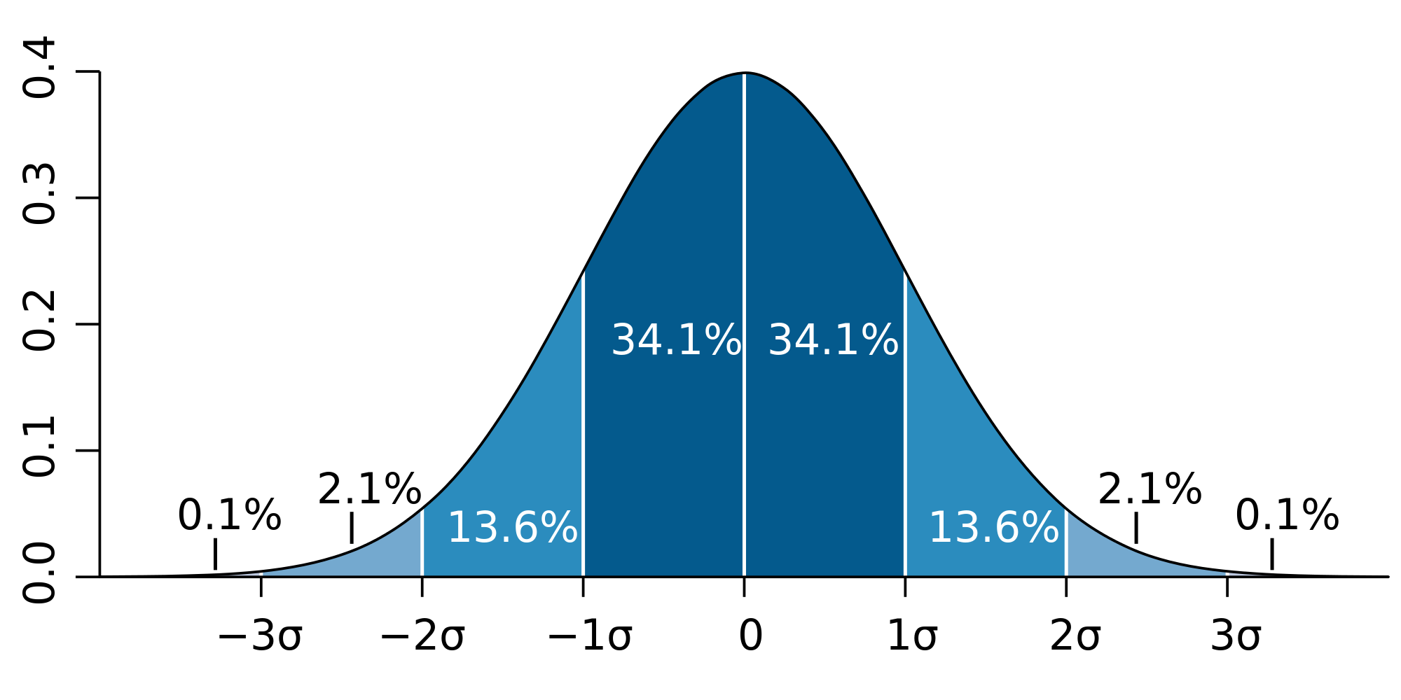
The denominator is just the normalization requirement discussed earlier. In general, the results of the various different measurements of \(x\) will be scattered around the expectation value \(\langle x\rangle\). The degree of scatter is parameterized by the quantity
\[ \begin{align} \sigma^2_x &= \int_{-\infty}^{\infty} \left(x-\langle x\rangle \right)^2 |\psi|^{ 2} dx \\[4pt] &\equiv \langle x^2\rangle -\langle x\rangle^{2}, \label{4.3.9} \end{align} \]
which is known as the variance of \(x\). The square-root of this quantity, \(\sigma_x\), is called the standard deviation of \(x\). We generally expect the results of measurements of \(x\) to lie within a few standard deviations of the expectation value (Figure \(\PageIndex{1}\)).
For a particle in a box in its ground state, calculate the expectation value of the
- position,
- the linear momentum,
- the kinetic energy, and
- the total energy
Solution
First the wavefunction needs to be defined. From the particle in the box solutions, the ground state wavefunction (\(n=1\) is
\[\psi = \sqrt{\dfrac{2}{L}} \sin \left ( \dfrac{\pi x}{L} \right ) \nonumber \]
We can confirm that the wavefunction is normalized.
\[\int \psi^* \psi \, d\tau = \int_{0}^{L} \sqrt{\dfrac{2}{L}} \sin \left ( \dfrac{\pi x}{L} \right ) \sqrt{\dfrac{2}{L}} \sin \left ( \dfrac{\pi x}{L} \right ) \, dx = 1 \nonumber\]
Hence, the Equation \(\ref{4.3.7}\) is the relevant equation to use.
The expectation value of the position is:
\[ \begin{align*} \left \langle x \right \rangle &= \int \psi^* x \psi \, d\tau = \int_{0}^{L} \sqrt{\dfrac{2}{L}} x \sin \left ( \dfrac{\pi x}{L} \right ) \sqrt{\dfrac{2}{L}} \sin \left ( \dfrac{\pi x}{L} \right ) \, dx \\[4pt] &=\dfrac{2}{L} \int_{0}^{L} x \sin^2 \left ( \dfrac{\pi x}{L} \right ) \, dx \\[4pt] &= \dfrac{L}{2} \end{align*}\]
The expectation value of the momentum is:
\[ \begin{align*} \left \langle p \right \rangle &= \int \psi^* \hat{p} \psi \, d\tau =\int_{0}^{L} \sqrt{\dfrac{2}{L}} \sin \left ( \dfrac{\pi x}{L} \right ) \left ( -i\hbar \dfrac{d}{dx} \right ) \sqrt{\dfrac{2}{L}} \sin \left ( \dfrac{\pi x}{L} \right ) \, dx \\[4pt] &= \dfrac{2i\hbar\pi}{L^2} \int_{0}^{L} \sin \left ( \dfrac{\pi x}{L} \right ) \cos \left ( \dfrac{\pi x}{L} \right ) \, dx \\[4pt] &= 0 \end{align*}\]
The expectation value of the kinetic energy is:
\[ \begin{align*} \left \langle T \right \rangle &= \int \psi^* \hat{K} \psi \, d\tau = \dfrac{2}{L} \int_{0}^{L} \sin \left ( \dfrac{\pi x}{L} \right ) \left ( -\dfrac{\hbar^2}{2m} \dfrac{\partial^2}{\partial x^2} \right ) \sin \left ( \dfrac{\pi x}{L} \right ) \, dx \\[4pt] &= \dfrac{\hbar^2 \pi^2}{2mL^2} \dfrac{2}{L} \int_{0}^{L} \sin^2 \left ( \dfrac{\pi x}{L} \right ) \, dx \\[4pt] &= \dfrac{\hbar^2 \pi^2}{2mL^2} \end{align*}\]
A position "on average" is in the middle of the box (L/2). It has equal probability of traveling towards the left or right, so the average momentum and velocity must be zero. The average kinetic energy must be equal to the total energy of the ground state of the particle in the box, as there is no other energy component (i.e, \(V=0\)).
Expanding the Wavefunction
It is also possible to demonstrate that the eigenstates of an operator attributed to a observable form a complete set (i.e., that any general wavefunction can be written as a linear combination of these eigenstates). However, the proof is quite difficult, and we shall not attempt it here.
In summary, given an operator \(\hat{A}\), any general wavefunction, \(\psi(x)\), can be written
\[\psi = \sum_{i}c_i \psi_i\label{4.3.9A}\]
where the \(c_i\) are complex weights, and the \(\psi(x)\) are the properly normalized (and mutually orthogonal) eigenstates of \(\hat{A}\): i.e.,
\[A \psi_i = a_i \psi_i \label{4.3.10}\]
where \(a_i\) is the eigenvalue corresponding to the eigenstate \(\psi_i\), and
\[\int_{-\infty}^\infty \psi_i^\ast \psi_j dx = \delta_{ij}. \label{4.3.11}\]
Here, \(\delta_{ij}\) is called the Kronecker delta-function, and takes the value unity when its two indices are equal, and zero otherwise. It follows from Equations \(\ref{4.3.8}\) and \(\ref{4.3.11}\) that
\[ c_i = \int_{-\infty}^\infty \psi_i^\ast \psi dx. \label{4.3.12}\]
Thus, the expansion coefficients in Equation \(\ref{4.3.12}\) are easily determined, given the wavefunction \(\psi\) and the eigenstates \(\psi_i\). Moreover, if \(\psi\) is a properly normalized wavefunction then Equations \(\ref{4.3.8}\) and \(\ref{4.3.11}\) yield
\[ \sum_i \vert c_i\vert^2 =1. \label{4.3.13}\]
Wave function collapse is said to occur when a wave function—initially in a superposition of several eigenstates—appears to reduce to a single eigenstate (by "observation"). A particle (or a system in general) can be found in a given state \(\psi(x,t)\). Suppose now a measurement is performed on the wavefuction to characterize a specific property of the system. Mathematically, an operator \(\hat{A}\) is associated with this measurement process, which you suppose has a complete orthonormal set of eigenvalues:
\[\{ \psi_i \}\]
that is typically an infinite set of functionals that depend on quantum number \(n\). The wavefunction \(\Psi\) can be expand and a set of basis functions can be selected to specifies the wavefunction is the coefficients \(\{c_n\}\) of the expansion. Therefore, if the system is perturbed, then your wavefunction will have another set of coefficients \(\{c'_n\}\).
Contributors
Richard Fitzpatrick (Professor of Physics, The University of Texas at Austin)
- Wikiversity
https://farside.ph.utexas.edu/teachi..es/node93.html