3.5: The Energy of a Particle in a Box is Quantized

The particle in the box model system is the simplest non-trivial application of the Schrödinger equation, but one which illustrates many of the fundamental concepts of quantum mechanics. For a particle moving in one dimension (again along the x- axis), the Schrödinger equation can be written

\[-\dfrac{\hbar^2}{2m}\psi {}''(x)+ V (x)\psi (x) = E \psi (x)\label{3.5.1}\]

Assume that the particle can move freely between two endpoints \(x = 0\) and \(x = L\), but cannot penetrate past either end. This is equivalent to a potential energy dependent on x with

\[V(x)=\begin{cases}
0 & 0\leq x\leq L \\
\infty & x< 0 \; and\; x> L \end{cases}\label{3.5.2}\]

This potential is represented in Figure \(\ref{3.5.1}\). The infinite potential energy constitutes an impenetrable barrier since the particle would have an infinite potential energy if found there, which is clearly impossible.

Figure \(\PageIndex{1}\): The barriers outside a one-dimensional box have infinitely large potential, while the interior of the box has a constant, zero potential. (CC-BY 4.0; OpenStax).

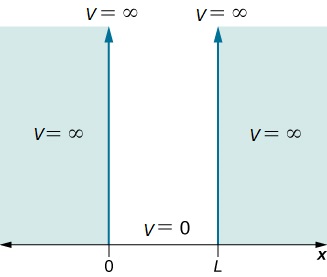
The particle is thus bound to a "potential well" since the particle cannot penetrate beyond \(x = 0\) or \(x = L\)

\[\psi (x)=0\; \; \; for \; \; x<0\; \; and\; \; x>L\label{3.5.3}\]

By the requirement that the wavefunction be continuous, it must be true as well that

\[\psi (0)=0\; \; \; and\; \; \; \psi (L)=0\label{3.5.4}\]

which constitutes a pair of boundary conditions on the wavefunction within the box. Inside the box, \(V(x) = 0\), so the Schrödinger equation reduces to the free-particle form:

\[-\dfrac{\hbar^2}{2m}\psi{}''(x)=E\psi (x) \label{3.5.5}\]

with \( 0\leq x\leq L\).

We again have the differential equation

\[\psi {}''(x) +k^2\psi (x)=0 \label{3.5.6}\]

with

\[k^2=2mE/\hbar^2 \label{3.5.6a}\]

The general solution can be written

\[\psi (x)=A\: \sin\; kx\,+\, B\: \cos\; kx\label{3.5.7}\]

where \(A\) and \(B\) are constants to be determined by the boundary conditions in Equation \(\ref{3.5.4}\). By the first condition, we find

\[\psi (0)=A\, \sin\, 0\, +\, B\, \cos\, 0\, =\, B\,= 0\label{3.5.8}\]

The second boundary condition at \(x = L\) then implies

\[\psi (a)=A\, \sin\, kL\,=\, 0\label{3.5.9}\]

It is assumed that \(A \neq 0\), for otherwise \(\psi(x)\) would be zero everywhere and the particle would disappear (i.e., the trivial solution). The condition that \(\sin kx = 0\) implies that

\[kL\, =\, n\pi \label{3.5.10}\]

where \(n\) is a integer, positive, negative or zero. The case \(n = 0\) must be excluded, for then \(k = 0\) and again \(\psi(x)\) would vanish everywhere. Eliminating \(k\) between Equation \(\ref{3.5.6}\) and \(\ref{3.5.10}\), we obtain

\[E_{n}=\dfrac{\hbar^2\pi^2}{2mL^2}\, n^2=\dfrac{h^2}{8mL^2}n^2 \label{3.5.11}\]

with \(n=1,2,,3...\).

These are the only values of the energy which allows solutions of the Schrö​dinger Equation \(\ref{3.5.5}\) consistent with the boundary conditions in Equation \(\ref{3.5.4}\). The integer \(n\), called a quantum number, is appended as a subscript on \(E\) to label the allowed energy levels. Negative values of \(n\) add nothing new because the energies in Equation \(\ref{3.5.11}\) depends on \(n^2\).

Figure \(\PageIndex{2}\): A plot of \(ψ_n(x)\) for the first four wavefunctions. (CC-BY 4.0; OpenStax).

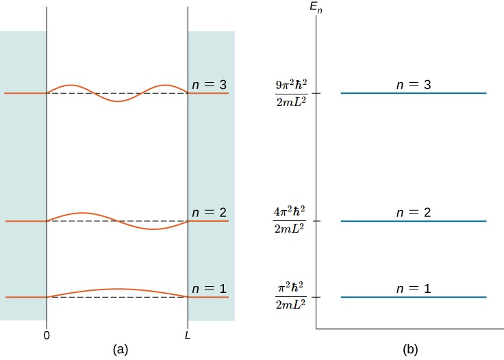
Figure \(\PageIndex{2}\) shows part of the energy-level diagram for the particle in a box. The occurrence of discrete or quantized energy levels is characteristic of a bound system, that is, one confined to a finite region in space. For the free particle, the absence of confinement allowed an energy continuum. Note that, in both cases, the number of energy levels is infinite-denumerably infinite for the particle in a box, but nondenumerably infinite for the free particle.

The particle in a box assumes its lowest possible energy when \(n = 1\), namely

\[E_{1}=\dfrac{h^2}{8mL^2}\label{3.5.12}\]

The state of lowest energy for a quantum system is termed its ground state.

Zero Point Energy

An interesting point is that \(E_{1} > 0\), whereas the corresponding classical system would have a minimum energy of zero. This is a recurrent phenomenon in quantum mechanics. The residual energy of the ground state, that is, the energy in excess of the classical minimum, is known as zero point energy. In effect, the kinetic energy, hence the momentum, of a bound particle cannot be reduced to zero. The minimum value of momentum is found by equating \(E_{1}\) to \(p^2/2m\), giving \(p_{min}\) = \(\pm h/2L\). This can be expressed as an uncertainty in momentum given by \(\Delta p\approx h/L\). Coupling this with the uncertainty in position, \(\Delta x\approx L\), from the size of the box, we can write

\[\Delta x\Delta p\approx h\label{3.5.13}\]

This is in accord with the Heisenberg uncertainty principle.

The particle-in-a-box eigenfunctions are given by Equation \(\ref{3.5.14}\), with \(B = 0\) and \(k = n\pi/L=a\), in accordance with Equation \(\ref{3.5.10}\)

\[\psi _{n}(x)=A\, \sin\dfrac{n\pi x}{L} \label{3.5.14} \]

with

\[n=1,2,3...\label{3.5.14a}\]

These, like the energies, can be labeled by the quantum number \(n\). The constant \(A\), thus far arbitrary, can be adjusted so that \(\psi _{n}(x)\) is normalized. The normalization condition is, in this case,

\[\int_{0}^{a}\begin{bmatrix}\psi_{n}(x) \end{bmatrix}^2\,dx=1\label{3.5.15}\]

the integration running over the domain of the particle \(0\leq x\leq a\). Substituting Equation \(\ref{3.5.14}\) into Equation \(\ref{3.5.15}\),

\[\begin{align} A^2\: \int_{0}^{L}\, \sin^2\, \dfrac{n\pi x}{L}dx &=A^2\dfrac{L}{n\pi}\int_{0}^{n\pi}\sin^2\, \theta \,d\theta \\[4pt] &=A^2\dfrac{L}{2}=1\label{3.5.16} \end{align}\]

We have made the substitution \(\theta=n\pi x/L\) and used the fact that the average value of \(\sin^2 \theta\) over an integral number of half wavelengths equals 1/2 (alternatively, one could refer to standard integral tables). From Equation \(\ref{3.5.16}\), we can identify the general normalization constant

\[A = \sqrt{ \dfrac{2}{L}}\]

for all values of \(n\). Finally we can write the normalized eigenfunctions:

\[\psi _{n}(x)=\sqrt{\dfrac{2}{L}} \sin \dfrac{n\pi x}{L} \label{3.5.17} \]

with

\[n=1,2,3...\label{3.5.17b}\]

The first few eigenfunctions and the corresponding probability distributions are plotted in Figure \(\PageIndex{3}\). There is a close analogy between the states of this quantum system and the modes of vibration of a violin string. The patterns of standing waves on the string are, in fact, identical in form with the wavefunctions in Equation \(\ref{3.5.17}\).

Figure \(\PageIndex{3}\): The probability density distribution \(|\psi_n(x)|^2\) for a quantum particle in a box for: (a) the ground state, \(n = 1\); (b) the first excited state, \(n = 2\); and, (c) the nineteenth excited state, \(n = 20\). (CC-BY 4.0; OpenStax).

Nodes and Curvature

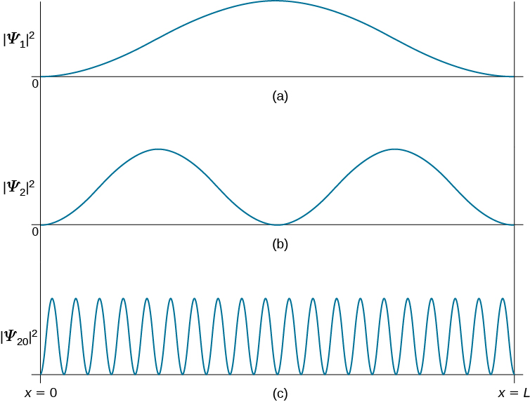
A significant feature of the particle-in-a-box quantum states is the occurrence of nodes. These are points, other than the two end points (which are fixed by the boundary conditions), at which the wavefunction vanishes. At a node there is exactly zero probability of finding the particle. The nth quantum state has, in fact, \(n-1\) nodes. It is generally true that the number of nodes increases with the energy of the quantum state, which can be rationalized by the following qualitative argument. As the number of nodes increases, so does the number and the steepness of the 'wiggles' in the wavefunction. It's like skiing down a slalom course. Accordingly, the average curvature, given by the second derivative, must increase. But the second derivative is proportional to the kinetic energy operator. Therefore, the more nodes, the higher the energy. This will prove to be an invaluable guide in more complex quantum systems.

Example \(\PageIndex{1}\): Excited State Probabilities

For a particle in a one-dimensional box of length \(L\), the second excited state wavefunction (\(n=3\)) is

\[\psi_3=\sqrt{\dfrac{2}{L}}\sin{\dfrac{3\pi x}{L}} \nonumber\]

1. What is the probability that the particle is in the left half of the box?
2. What is the probability that the particle is in the middle third of the box?

Solution

Probability that the particle will be found between \(a\) and \(b\) is

$$P(a,b)=\int^b_a \psi^2\,dx \nonumber $$

For this problem,

$$\psi_3=\sqrt{\dfrac{2}{L}}\sin{\dfrac{3\pi x}{L}} \nonumber $$

therefore,

\[ \begin{align*} P(a,b) &=\dfrac{2}{L} \int^b_a \sin^2 {\dfrac{3\pi x}{L}}\,dx \\ &=\left.\dfrac{2}{L}\left(\dfrac{x}{2}-\dfrac{L\sin \left( \dfrac{6\pi x}{L}\right)}{12\pi} \right) \right|^b_a \\[4pt] &=\dfrac{b-a}{L}-\dfrac{1}{6\pi} \left[ \sin \left(\dfrac{6\pi b}{L}\right) - \sin \left( \dfrac{6\pi a}{L} \right) \right] \end{align*}\]

(a) The probability that the particle is in the left half of the box is

\[ \begin{align*} P\left(0,\dfrac{L}{2}\right) &=\dfrac{\dfrac{L}{2}-0}{L}-\dfrac{1}{6\pi}\left[ \sin \left( \dfrac{6\pi \left(\dfrac{L}{2}\right)}{L}\right) - \sin \left( \dfrac{6\pi (0)}{L}\right) \right] \\[4pt] &= \dfrac{1}{2} \end{align*}\]

(b) The probability that the particle is in the middle third of the box

\[ \begin{align*} P\left(\dfrac{L}{3},\dfrac{2L}{3}\right) &=\dfrac{\dfrac{2L}{3}-\dfrac{L}{3}}{L}-\dfrac{1}{6\pi}\left[{\sin {\dfrac{6\pi \left(\dfrac{2L}{3}\right)}{L} }-\sin {\dfrac{6\pi \left(\dfrac{L}{3}\right) }{L} }}\right] \\[4pt] &=\dfrac{1}{3} \end{align*}\]

Exercise \(\PageIndex{1}\): ground State Probability

For a particle in a one-dimensional box, the ground state wave function is

\[\psi_1 = \sqrt{\dfrac{2}{L}} \sin\dfrac{x\pi}{L} \nonumber\]

What is the probability that the particle is in the left half of the box in the ground state?

Answer

\[ \begin{align} P\left(0,\frac{L}{2}\right) &= \dfrac{2}{L} \int^{\frac{L}{2}}_0 \sin^2 \dfrac{x\pi}{L} dx \nonumber \nonumber\\ &=\dfrac{2}{L} \dfrac{\dfrac{L\pi}{L}+\sin 0+\sin \dfrac{L\pi}{L}}{\dfrac{4\pi}{L}} \nonumber\\ &=\dfrac{1}{2} \nonumber \end{align} \nonumber\]

This is the same answer as for the \(\psi_3\) state in Example \(\PageIndex{1}\). This is because the eigenstate squared (.e., probability density) for the particle in a 1D box will always be symmetric around the center of the box. So there will be equal probability to be on either side (i.e., no side is favored).

Time dependence and Complex Behavior of wavefunctions

Recall that the time-dependence of the wavefunction with time-independent potential was discussed in Section 3.1 and is expressed as

\[\Psi(x,t)=\psi(x)e^{-iEt / \hbar}\]

so for the particle in a box, these are

\[\psi _{n}(x)=\sqrt{\dfrac{2}{L}} \sin \dfrac{n\pi x}{L} e^{-iE_nt / \hbar} \label{PIBtime} \]

with \(E_n\) given by Equation \ref{3.5.11}.

The phase part of Equation \ref{PIBtime} can be expanded into a real part and a complex components. So the total wavefunction for a particle in a box is

\[\Psi(x,t)= \underbrace{\left(\sqrt{\dfrac{2}{L}} \sin \dfrac{n\pi x}{L}\right) \left(\cos \dfrac{E_nt}{\hbar}\right)}_{\text{real part}} - \underbrace{i \left(\, \sqrt{\dfrac{2}{L}} \sin \dfrac{n\pi x}{L} \right) \left(\sin \dfrac{E_nt}{\hbar} \right) }_{\text{imaginary part}}\]

which can be simplified (slightly) to

\[\Psi(x,t)= \underbrace{\left(\sqrt{\dfrac{2}{L}} \sin \dfrac{n\pi x}{L}\right) \left(\cos \dfrac{E_nt}{\hbar}\right)}_{\text{real part}} - \underbrace{i \left(\, \sqrt{\dfrac{2}{L}} \sin \dfrac{n\pi x}{L} \right) \left(\cos \dfrac{E_nt}{\hbar} - \dfrac{\pi}{2} \right) }_{\text{imaginary part}}\]

As discussed previously, the imaginary part of the total wavefunction oscillates out of phase by \(π/2\) with respect to the real part (we call this "out of phase"). This is demonstrated in the time-dependent behavior of the first three eigenfunctions in Figure \(\PageIndex{4}\).

Figure \(\PageIndex{5}\): Some trajectories of a particle in a box according to Newton's laws of classical mechanics (A), and according to the Schrödinger equation of quantum mechanics (B-F). In (B-D), the horizontal axis is position, and the vertical axis is the real part (blue) and imaginary part (red) of the wavefunction. The states (B,C,D) are energy eigenstates. (Public Domain; Sbyrnes321 via Wikipedia).

Note that as \(n\) increased, the energy of the wavefunction increases (Equation \ref{3.5.11}) and both the number of nodes and antinodes increase and the frequency of oscillation of the wavefunction increases.

It is generally true in quantum systems (not just for particles in boxes) that the number of nodes in a wavefunction increases with the energy of the quantum state.

Orthonormality

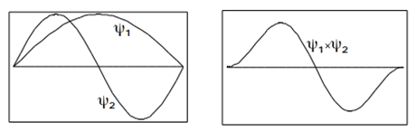
Another important property of the eigenfunctions in Equation \(\ref{3.5.17}\) applies to the integral over a product of two different eigenfunctions. It is easy to see from Figure \(\PageIndex{5}\) that the integral

\[\int_{0}^{a}\psi _{2}(x)\psi _{1}(x)dx=0 \label{3.5.18}\]

Figure \(\PageIndex{5}\): Product of \(n=1\) and \(n=2\) eigenfunctions.

To prove this result in general, use the trigonometric identity

\[\sin\,\alpha \: \sin\, \beta =\dfrac{1}{2}\begin{bmatrix}\cos(\alpha -\beta )-\cos(\alpha +\beta )\end{bmatrix} \label{trig}\]

to show that

\[\int_{0}^{L}\psi _{m}(x)\psi _{n}(x)dx=0\: \: \: if\: \: \: m \neq n\label{3.5.19}\]

This property is called orthogonality​. We will show in the next Chapter, that this is a general result from quantum-mechanical eigenfunctions. The normalization (Equation \(\ref{3.5.18}\)) together with the orthogonality (Equation \(\ref{3.5.19}\)) can be combined into a single relationship

\[\int_{0}^{L}\psi _{m}(x)\psi _{n}(x)dx=\delta _{mn}\label{3.5.20}\]

In terms of the Kronecker delta

\[\delta _{mn}=\begin{cases}
1 & \text{if} \,\, m=n \\[4pt]
0 & \text{if} \,\, m\neq n \end{cases}\label{3.5.21}\]

A set of functions \(\begin{Bmatrix}\psi_{n}\end{Bmatrix}\) which obeys Equation \(\ref{3.5.20}\) is called orthonormal.

Example \(\PageIndex{2}\)

Evaluate

1. \(\langle \psi_3| \psi_3 \rangle \)
2. \(\langle \psi_4| \psi_4 \rangle \)
3. \(\langle \psi_3| \psi_4 \rangle \)
4. \(\langle \psi_4| \psi_4 \rangle \)

for the normalized wavefunctions:

\[|\psi_3 \rangle = \sqrt{ \dfrac{2}{L}} \sin\dfrac{3\pi x}{L} \nonumber \]

and

\[|\psi_4 \rangle = \sqrt{ \dfrac{2}{L}} \sin\dfrac{4\pi x}{L}\nonumber\]

Strategy

These are four different integrals and we can solve them directly or use orthonormality (Equation \ref{3.5.21}) to evaluate.

a.

\[ \begin{align*} \langle \psi_3| \psi_3 \rangle &= \int_{-\infty}^{+\infty} \left( \sqrt{ \dfrac{2}{L}} \sin\dfrac{3\pi x}{L} \right)\left( \sqrt{ \dfrac{2}{L}} \sin\dfrac{3\pi x}{L} \right)\, dx \\[4pt] &= \dfrac{2}{L} \int_{-\infty}^{+\infty} \sin^2 \dfrac{3\pi x}{L} \, dx \end{align*}\]

This is an integration over an even function, so it cannot be tossed out via symmetry. We can use the Trigonometry relationship in Equation \ref{trig} to get

\[ \dfrac{2}{L} \int_{-\infty}^{+\infty} \sin^2 \dfrac{3\pi x}{L} \, dx = \dfrac{2}{L} \int_{-\infty}^{+\infty} \dfrac{1}{2} \left(1 - \cos \dfrac{6\pi x}{L}\right) \, dx \nonumber \]

and we can continue the fun. However, there is no need. Since the we can recognize that \(\langle \psi_3| \psi_3 \rangle \) is 1 by the normalization criteria which is folded into the orthonormal criteria (Equation \ref{3.5.21}).

Therefore \(\langle \psi_3| \psi_3 \rangle = 1\).

b.

\[ \begin{align*} \langle \psi_4| \psi_4 \rangle &= \int_{-\infty}^{+\infty} \left( \sqrt{ \dfrac{2}{L}} \sin\dfrac{4\pi x}{L} \right)\left( \sqrt{ \dfrac{2}{L}} \sin\dfrac{4\pi x}{L} \right)\, dx \\[4pt] &= \dfrac{2}{L} \int_{-\infty}^{+\infty} \sin^2 \dfrac{4\pi x}{L} \, dx \end{align*}\]

We can expand and solve, but again there is no need. The wavefunctions are normalized therefore \(\langle \psi_4| \psi_4 \rangle = 1\).

c.

\[ \begin{align*} \langle \psi_3| \psi_4 \rangle &= \int_{-\infty}^{+\infty} \left( \sqrt{ \dfrac{2}{L}} \sin\dfrac{3\pi x}{L} \right)\left( \sqrt{ \dfrac{2}{L}} \sin\dfrac{4\pi x}{L} \right)\, dx \\[4pt] &= \dfrac{2}{L} \int_{-\infty}^{+\infty} \sin^2 \dfrac{4\pi x}{L} \, dx \end{align*}\]

We can expand this integral and evaluate, but since the integrand is odd, this integral is zero. Alternatively, we can use the orgonality criteria into the greater orthonormal criteria (Equation \ref{3.5.21}).

d.

\[ \begin{align*} \langle \psi_4| \psi_3 \rangle &= \int_{-\infty}^{+\infty} \left( \sqrt{ \dfrac{2}{L}} \sin\dfrac{4\pi x}{L} \right)\left( \sqrt{ \dfrac{2}{L}} \sin\dfrac{3\pi x}{L} \right)\, dx \\[4pt] &= \dfrac{2}{L} \int_{-\infty}^{+\infty} \sin^2 \dfrac{4\pi x}{L} \, dx \end{align*}\]

We can expand this integral and evaluate, but since the integrand is odd, this integral is zero. Alternatively, we can use the orthogonality criteria into the greater orthonormal criteria (Equation \ref{3.5.21}).

However, since the wavefunctions are real, then

\[\langle \psi_4| \psi_3 \rangle = \langle \psi_3| \psi_4 \rangle \nonumber \]

which also means

\[\langle \psi_4| \psi_3 \rangle = 0 \nonumber\]

from the results of section c.

Contributors

• Seymour Blinder (Professor Emeritus of Chemistry and Physics at the University of Michigan, Ann Arbor)