
1: The simplest chemical bond: The \(H_2^+\) Ion
- Page ID
- 20848

\( \newcommand{\vecs}[1]{\overset { \scriptstyle \rightharpoonup} {\mathbf{#1}} } \)
\( \newcommand{\vecd}[1]{\overset{-\!-\!\rightharpoonup}{\vphantom{a}\smash {#1}}} \)
\( \newcommand{\id}{\mathrm{id}}\) \( \newcommand{\Span}{\mathrm{span}}\)
( \newcommand{\kernel}{\mathrm{null}\,}\) \( \newcommand{\range}{\mathrm{range}\,}\)
\( \newcommand{\RealPart}{\mathrm{Re}}\) \( \newcommand{\ImaginaryPart}{\mathrm{Im}}\)
\( \newcommand{\Argument}{\mathrm{Arg}}\) \( \newcommand{\norm}[1]{\| #1 \|}\)
\( \newcommand{\inner}[2]{\langle #1, #2 \rangle}\)
\( \newcommand{\Span}{\mathrm{span}}\)
\( \newcommand{\id}{\mathrm{id}}\)
\( \newcommand{\Span}{\mathrm{span}}\)
\( \newcommand{\kernel}{\mathrm{null}\,}\)
\( \newcommand{\range}{\mathrm{range}\,}\)
\( \newcommand{\RealPart}{\mathrm{Re}}\)
\( \newcommand{\ImaginaryPart}{\mathrm{Im}}\)
\( \newcommand{\Argument}{\mathrm{Arg}}\)
\( \newcommand{\norm}[1]{\| #1 \|}\)
\( \newcommand{\inner}[2]{\langle #1, #2 \rangle}\)
\( \newcommand{\Span}{\mathrm{span}}\) \( \newcommand{\AA}{\unicode[.8,0]{x212B}}\)
\( \newcommand{\vectorA}[1]{\vec{#1}} % arrow\)
\( \newcommand{\vectorAt}[1]{\vec{\text{#1}}} % arrow\)
\( \newcommand{\vectorB}[1]{\overset { \scriptstyle \rightharpoonup} {\mathbf{#1}} } \)
\( \newcommand{\vectorC}[1]{\textbf{#1}} \)
\( \newcommand{\vectorD}[1]{\overrightarrow{#1}} \)
\( \newcommand{\vectorDt}[1]{\overrightarrow{\text{#1}}} \)
\( \newcommand{\vectE}[1]{\overset{-\!-\!\rightharpoonup}{\vphantom{a}\smash{\mathbf {#1}}}} \)
\( \newcommand{\vecs}[1]{\overset { \scriptstyle \rightharpoonup} {\mathbf{#1}} } \)
\( \newcommand{\vecd}[1]{\overset{-\!-\!\rightharpoonup}{\vphantom{a}\smash {#1}}} \)
\(\newcommand{\avec}{\mathbf a}\) \(\newcommand{\bvec}{\mathbf b}\) \(\newcommand{\cvec}{\mathbf c}\) \(\newcommand{\dvec}{\mathbf d}\) \(\newcommand{\dtil}{\widetilde{\mathbf d}}\) \(\newcommand{\evec}{\mathbf e}\) \(\newcommand{\fvec}{\mathbf f}\) \(\newcommand{\nvec}{\mathbf n}\) \(\newcommand{\pvec}{\mathbf p}\) \(\newcommand{\qvec}{\mathbf q}\) \(\newcommand{\svec}{\mathbf s}\) \(\newcommand{\tvec}{\mathbf t}\) \(\newcommand{\uvec}{\mathbf u}\) \(\newcommand{\vvec}{\mathbf v}\) \(\newcommand{\wvec}{\mathbf w}\) \(\newcommand{\xvec}{\mathbf x}\) \(\newcommand{\yvec}{\mathbf y}\) \(\newcommand{\zvec}{\mathbf z}\) \(\newcommand{\rvec}{\mathbf r}\) \(\newcommand{\mvec}{\mathbf m}\) \(\newcommand{\zerovec}{\mathbf 0}\) \(\newcommand{\onevec}{\mathbf 1}\) \(\newcommand{\real}{\mathbb R}\) \(\newcommand{\twovec}[2]{\left[\begin{array}{r}#1 \\ #2 \end{array}\right]}\) \(\newcommand{\ctwovec}[2]{\left[\begin{array}{c}#1 \\ #2 \end{array}\right]}\) \(\newcommand{\threevec}[3]{\left[\begin{array}{r}#1 \\ #2 \\ #3 \end{array}\right]}\) \(\newcommand{\cthreevec}[3]{\left[\begin{array}{c}#1 \\ #2 \\ #3 \end{array}\right]}\) \(\newcommand{\fourvec}[4]{\left[\begin{array}{r}#1 \\ #2 \\ #3 \\ #4 \end{array}\right]}\) \(\newcommand{\cfourvec}[4]{\left[\begin{array}{c}#1 \\ #2 \\ #3 \\ #4 \end{array}\right]}\) \(\newcommand{\fivevec}[5]{\left[\begin{array}{r}#1 \\ #2 \\ #3 \\ #4 \\ #5 \\ \end{array}\right]}\) \(\newcommand{\cfivevec}[5]{\left[\begin{array}{c}#1 \\ #2 \\ #3 \\ #4 \\ #5 \\ \end{array}\right]}\) \(\newcommand{\mattwo}[4]{\left[\begin{array}{rr}#1 \amp #2 \\ #3 \amp #4 \\ \end{array}\right]}\) \(\newcommand{\laspan}[1]{\text{Span}\{#1\}}\) \(\newcommand{\bcal}{\cal B}\) \(\newcommand{\ccal}{\cal C}\) \(\newcommand{\scal}{\cal S}\) \(\newcommand{\wcal}{\cal W}\) \(\newcommand{\ecal}{\cal E}\) \(\newcommand{\coords}[2]{\left\{#1\right\}_{#2}}\) \(\newcommand{\gray}[1]{\color{gray}{#1}}\) \(\newcommand{\lgray}[1]{\color{lightgray}{#1}}\) \(\newcommand{\rank}{\operatorname{rank}}\) \(\newcommand{\row}{\text{Row}}\) \(\newcommand{\col}{\text{Col}}\) \(\renewcommand{\row}{\text{Row}}\) \(\newcommand{\nul}{\text{Nul}}\) \(\newcommand{\var}{\text{Var}}\) \(\newcommand{\corr}{\text{corr}}\) \(\newcommand{\len}[1]{\left|#1\right|}\) \(\newcommand{\bbar}{\overline{\bvec}}\) \(\newcommand{\bhat}{\widehat{\bvec}}\) \(\newcommand{\bperp}{\bvec^\perp}\) \(\newcommand{\xhat}{\widehat{\xvec}}\) \(\newcommand{\vhat}{\widehat{\vvec}}\) \(\newcommand{\uhat}{\widehat{\uvec}}\) \(\newcommand{\what}{\widehat{\wvec}}\) \(\newcommand{\Sighat}{\widehat{\Sigma}}\) \(\newcommand{\lt}{<}\) \(\newcommand{\gt}{>}\) \(\newcommand{\amp}{&}\) \(\definecolor{fillinmathshade}{gray}{0.9}\)The \(H_2^+\) molecule ion is an example of a simple one-electron problem that can be solved exactly and leads to the energy eigenfunctions associated with an actual chemical bond. In fact, this molecule is the only one for which analytical solutions are known. The actual solution is complicated, so we will not carry it out to completion, but here we will outline how it is done:
Setting up the Hamiltonian
H2+ consists of two protons and one electron. Choose a coordinate system as follows:
![]()
![]()
|
|
|
|
|
|
|
|

|
![]()
Here, r denotes the position of the electron. For now we will assume that the protons remain fixed in space with a distance R between them. The coordinate system is chosen so that both protons lie on the z-axis.
Proton positions are ![]() ,
, ![]()
![]()
![]()
Hence, the Hamiltonian is:

Eigenfunctions of H satisfy


The potential

is not a central-symmetric potential. Hence,
![]()
so angular momentum is not conserved. But we do have cylindrical symmetry about the z-axis. Hence, the z-component of angular momentum is a constant of the motion and can be shown to satisfy:
![]()
![]()
Therefore, eigenfunctions of H are also eigenfunctions of ![]() .
.
Recall ![]() can be defined in terms of an angle
can be defined in terms of an angle ![]() about the z-axis.
about the z-axis. ![]()
 | |||
|
|
![]()
|
|
|
|
|
![]()
That is, the angle is defined as the angle between the projection of the vector r onto the x-y plane and the positive x-axis.
![]()
Eigenfunctions satisfy
![]()
![]()
![]()
However, periodicity in the angle φ requires
![]()
![]()
![]()
which is true only if
![]()
![]()
![]()
indicating that the eigenvalues of Lz are discrete multiplies of ħ
![]()
In addition, the eigenfunctions are required to be properly normalized, hence:

![]()
![]()
![]()
We still need two other coordinates to specify the wave function.
We cannot use the spherical coordinates ![]() because we do not have a central potential, i.e. one that only depends on the distance of the electron from the origin. Rather, the potential for the H2+ molecule ion depends on the distance of the electron from two points representing the two protons.
because we do not have a central potential, i.e. one that only depends on the distance of the electron from the origin. Rather, the potential for the H2+ molecule ion depends on the distance of the electron from two points representing the two protons.
We cannot take advantage of cylindrical coordinates because the potential is not a single function of those coordinates.
Such problems can be treated using confocal elliptic coordinates defined as follows
![]()
![]()
in terms of r this is


Solving for ra and rb gives
![]()
![]()
Hence, the potential becomes:
![]()
We can also derive an expression for Ñ2 can also be derived in terms of m, n and φ via the chain rule:
![]()
![]()
etc.
We find:

The Schrödinger (eigenvalue) equation becomes:
![]()
Write
![]()
![]()
Multiply through by ![]()
![]()

![]()
If we let
![]()
then, the equation separates:
![]()


Let
![]()
![]()
The equation is now separable in m and n. Hence, we can choose:
![]()
Also, write
![]()
![]()
Hence, substitution of the separable form into the equation gives


The constant A reflects the fact that the left side is a function of m alone while the right side is a function of n alone. Since they are equal to each other, they must both be equal to the same constant A. The constant A is known as the separation constant.
Hence, we arrive at two equations for the functions M and N:


We need to solve these equations for ![]() and
and ![]() and obtain conditions on allowed values of P (meaning E) and A.
and obtain conditions on allowed values of P (meaning E) and A.
The conditions on P and A will lead to two new quantum numbers denoted ![]() and n so that
and n so that
![]()
However, unlike for hydrogen, there is no nice, simple closed-form expression, only implicit equations.
Solutions are of the form
![]()
![]()
where
![]()
and
![]() .
.
The contour plots below represent the exact solutions for different values of R:


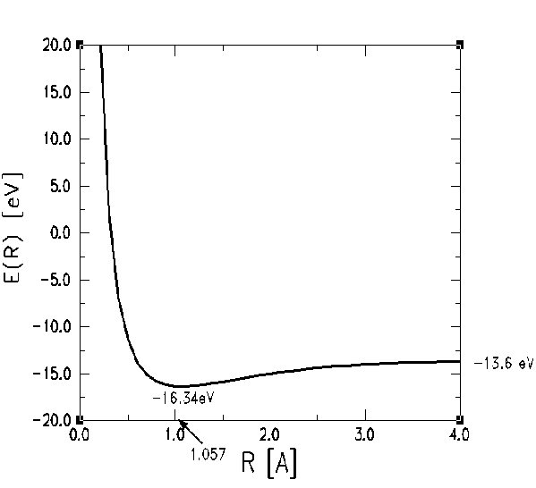
A plot of the energy of the system as a function of R is shown below: