
12: Molecular geometry, coordinates, and dipole moments
- Page ID
- 17132

\( \newcommand{\vecs}[1]{\overset { \scriptstyle \rightharpoonup} {\mathbf{#1}} } \)
\( \newcommand{\vecd}[1]{\overset{-\!-\!\rightharpoonup}{\vphantom{a}\smash {#1}}} \)
\( \newcommand{\id}{\mathrm{id}}\) \( \newcommand{\Span}{\mathrm{span}}\)
( \newcommand{\kernel}{\mathrm{null}\,}\) \( \newcommand{\range}{\mathrm{range}\,}\)
\( \newcommand{\RealPart}{\mathrm{Re}}\) \( \newcommand{\ImaginaryPart}{\mathrm{Im}}\)
\( \newcommand{\Argument}{\mathrm{Arg}}\) \( \newcommand{\norm}[1]{\| #1 \|}\)
\( \newcommand{\inner}[2]{\langle #1, #2 \rangle}\)
\( \newcommand{\Span}{\mathrm{span}}\)
\( \newcommand{\id}{\mathrm{id}}\)
\( \newcommand{\Span}{\mathrm{span}}\)
\( \newcommand{\kernel}{\mathrm{null}\,}\)
\( \newcommand{\range}{\mathrm{range}\,}\)
\( \newcommand{\RealPart}{\mathrm{Re}}\)
\( \newcommand{\ImaginaryPart}{\mathrm{Im}}\)
\( \newcommand{\Argument}{\mathrm{Arg}}\)
\( \newcommand{\norm}[1]{\| #1 \|}\)
\( \newcommand{\inner}[2]{\langle #1, #2 \rangle}\)
\( \newcommand{\Span}{\mathrm{span}}\) \( \newcommand{\AA}{\unicode[.8,0]{x212B}}\)
\( \newcommand{\vectorA}[1]{\vec{#1}} % arrow\)
\( \newcommand{\vectorAt}[1]{\vec{\text{#1}}} % arrow\)
\( \newcommand{\vectorB}[1]{\overset { \scriptstyle \rightharpoonup} {\mathbf{#1}} } \)
\( \newcommand{\vectorC}[1]{\textbf{#1}} \)
\( \newcommand{\vectorD}[1]{\overrightarrow{#1}} \)
\( \newcommand{\vectorDt}[1]{\overrightarrow{\text{#1}}} \)
\( \newcommand{\vectE}[1]{\overset{-\!-\!\rightharpoonup}{\vphantom{a}\smash{\mathbf {#1}}}} \)
\( \newcommand{\vecs}[1]{\overset { \scriptstyle \rightharpoonup} {\mathbf{#1}} } \)
\( \newcommand{\vecd}[1]{\overset{-\!-\!\rightharpoonup}{\vphantom{a}\smash {#1}}} \)
\(\newcommand{\avec}{\mathbf a}\) \(\newcommand{\bvec}{\mathbf b}\) \(\newcommand{\cvec}{\mathbf c}\) \(\newcommand{\dvec}{\mathbf d}\) \(\newcommand{\dtil}{\widetilde{\mathbf d}}\) \(\newcommand{\evec}{\mathbf e}\) \(\newcommand{\fvec}{\mathbf f}\) \(\newcommand{\nvec}{\mathbf n}\) \(\newcommand{\pvec}{\mathbf p}\) \(\newcommand{\qvec}{\mathbf q}\) \(\newcommand{\svec}{\mathbf s}\) \(\newcommand{\tvec}{\mathbf t}\) \(\newcommand{\uvec}{\mathbf u}\) \(\newcommand{\vvec}{\mathbf v}\) \(\newcommand{\wvec}{\mathbf w}\) \(\newcommand{\xvec}{\mathbf x}\) \(\newcommand{\yvec}{\mathbf y}\) \(\newcommand{\zvec}{\mathbf z}\) \(\newcommand{\rvec}{\mathbf r}\) \(\newcommand{\mvec}{\mathbf m}\) \(\newcommand{\zerovec}{\mathbf 0}\) \(\newcommand{\onevec}{\mathbf 1}\) \(\newcommand{\real}{\mathbb R}\) \(\newcommand{\twovec}[2]{\left[\begin{array}{r}#1 \\ #2 \end{array}\right]}\) \(\newcommand{\ctwovec}[2]{\left[\begin{array}{c}#1 \\ #2 \end{array}\right]}\) \(\newcommand{\threevec}[3]{\left[\begin{array}{r}#1 \\ #2 \\ #3 \end{array}\right]}\) \(\newcommand{\cthreevec}[3]{\left[\begin{array}{c}#1 \\ #2 \\ #3 \end{array}\right]}\) \(\newcommand{\fourvec}[4]{\left[\begin{array}{r}#1 \\ #2 \\ #3 \\ #4 \end{array}\right]}\) \(\newcommand{\cfourvec}[4]{\left[\begin{array}{c}#1 \\ #2 \\ #3 \\ #4 \end{array}\right]}\) \(\newcommand{\fivevec}[5]{\left[\begin{array}{r}#1 \\ #2 \\ #3 \\ #4 \\ #5 \\ \end{array}\right]}\) \(\newcommand{\cfivevec}[5]{\left[\begin{array}{c}#1 \\ #2 \\ #3 \\ #4 \\ #5 \\ \end{array}\right]}\) \(\newcommand{\mattwo}[4]{\left[\begin{array}{rr}#1 \amp #2 \\ #3 \amp #4 \\ \end{array}\right]}\) \(\newcommand{\laspan}[1]{\text{Span}\{#1\}}\) \(\newcommand{\bcal}{\cal B}\) \(\newcommand{\ccal}{\cal C}\) \(\newcommand{\scal}{\cal S}\) \(\newcommand{\wcal}{\cal W}\) \(\newcommand{\ecal}{\cal E}\) \(\newcommand{\coords}[2]{\left\{#1\right\}_{#2}}\) \(\newcommand{\gray}[1]{\color{gray}{#1}}\) \(\newcommand{\lgray}[1]{\color{lightgray}{#1}}\) \(\newcommand{\rank}{\operatorname{rank}}\) \(\newcommand{\row}{\text{Row}}\) \(\newcommand{\col}{\text{Col}}\) \(\renewcommand{\row}{\text{Row}}\) \(\newcommand{\nul}{\text{Nul}}\) \(\newcommand{\var}{\text{Var}}\) \(\newcommand{\corr}{\text{corr}}\) \(\newcommand{\len}[1]{\left|#1\right|}\) \(\newcommand{\bbar}{\overline{\bvec}}\) \(\newcommand{\bhat}{\widehat{\bvec}}\) \(\newcommand{\bperp}{\bvec^\perp}\) \(\newcommand{\xhat}{\widehat{\xvec}}\) \(\newcommand{\vhat}{\widehat{\vvec}}\) \(\newcommand{\uhat}{\widehat{\uvec}}\) \(\newcommand{\what}{\widehat{\wvec}}\) \(\newcommand{\Sighat}{\widehat{\Sigma}}\) \(\newcommand{\lt}{<}\) \(\newcommand{\gt}{>}\) \(\newcommand{\amp}{&}\) \(\definecolor{fillinmathshade}{gray}{0.9}\)Molecular geometry and coordinates
Consider a diatomic molecule AB. Imagine fixing this molecule at a very specific spatial location, as shown below:
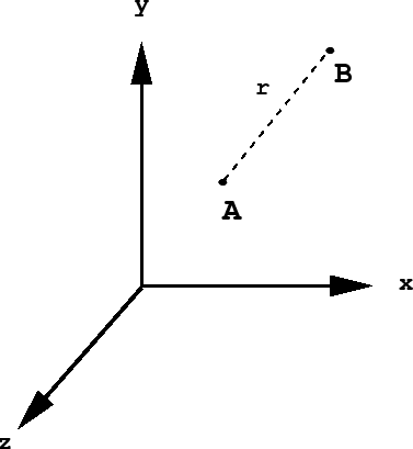
To locate the molecule so specifically, we would need to give the \(x\), \(y\), and \(z\) coordinates of each of its atoms, i.e.,
\[\begin{align*}(x_A ,y_A ,z_A) &= r_A\\ (x_B ,y_B ,z_B) &= r_B\end{align*}\]
which is a total of 6 numbers.
However, we note that the molecule looks the same, no matter where in space it is located. This is called translational invariance, and it implies that we can give only the coordinates of one of the atoms relative to the other, which is equivalent to giving the vector difference between \(r_B\) and \(r_A\) (or vice-versa), which we will call the vector \(r\):
which is only 3 numbers. This is the same as arbitrarily placing atom A at the origin of our \(xyz\) coordinate system.
We also note that the spatial orientation of the molecule is arbitrary, since the molecule looks the same at any viewing angle. For a diatomic, its orientation can be specified by giving two angles: the angle it makes with the z-axis and the angle of its projection onto the \(xy\) plane with the x-axis. The choice of these angles is arbitrary. This leaves only 1 number left, which is the distance between A and B, called the molecule's bond length.
\[\begin{align*}r &= |r|=\sqrt{x^2 +y^2 +z^2}\\ &= |r_b - r_A| = \sqrt{(x_B -x_A)^2 +(y_B -y_A)^2 +(z_B -z_A)^2}\end{align*}\]
This is an internal degree of freedom and is the only important number we need to give in order to convey the geometry of the diatomic.
In spite of this simplification, it is often necessary to specify all of the coordinates of the atoms in a molecule. Molecular modeling packages, which are becoming increasingly important in chemical research, require a full set of coordinates for each atom as input. Similarly, molecular data banks, such as the protein data bank (PDB) will give molecular structures as files of \(x\), \(y\), and \(z\) coordinates. Thus, being able to determine a set of coordinates given only bond lengths and bond angles, and conversely being able to determine bond lengths and angles from a set of coordinates is an extremely important skill. A few examples of how to do this will be illustrated below.
Example 1
The diatomic \(AB\). How do we determine a set of coordinates for \(AB\) given only its bond length \(r\). Since its absolute location in space and its orientation are arbitrary, any set of coordinates that reproduces the correct bond length will suffice. Thus, since a diatomic is linear, we may place it along one of the axes of our coordinate system with one of the atoms at the origin:
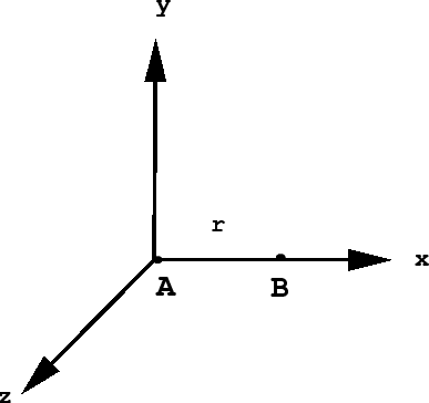
Now we see that the coordinates of atom \(A\) will simply be
and the coordinates of atom \(B\), since \(B\) lies on the x-axis a distance \(r\) away from \(A\), will be
Clearly, this set of coordinates reproduces the correct bond length:
\[|r_B -r_A|=\sqrt{r^2 +0^2 +0^2}=r\]
Thus, for the molecule \(HCl\), whose bond length is \(r=1.284 \ \stackrel{\circ}{A}\), a set of coordinates could be
\[\begin{align*}r_H &= (0,0,0)\\ r_Cl &= (1.284,0,0)\end{align*}\]
in \(\stackrel{\circ}{A}\). This is just one possibility. We could have chosen either atom to be at the origin (or anywhere else in space for that matter), and chosen the bond to lie along any axis (or not along any particular axis), as we choose, so long as the correct bond length is reproduced.
Example 2
Water, \(H_2 O\): The geometry of water is bent (we will see how to determine this later), with a bond angle of \(104.5^\circ\) and an \(OH\) bond length of approximately \(1.0 \ \stackrel{\circ}{A}\).
To determine a set of coordinates for \(H_2 O\), we note that the molecule is planar, so we may choose it to lie in the \(xy\) plane. We will place the oxygen at the origin with the hydrogens as shown below:
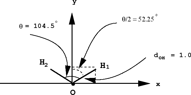
The coordinates of the oxygen can be written down immediately:
For each of the hydrogens, note that the y-axis bisects the angle, giving two right triangles. An \(OH\) bond forms the hypotenuse of one of these triangles, so that the \(x\) and \(y\) coordinates will be determined from the sine and cosine of the angle \(\theta /2\), as can be shown using simple trigonometry:
\[\begin{align*}r_{H_1} &= (d_{OH}sin\theta /2,d_{OH}cos\theta /2,0)=(0.7907,0.6122,0)\\ r_{H_2} &= (-d_{OH}sin\theta /2,d_{OH}cos\theta /2,0)=(-0.7907,0.6122,0) \end{align*}\]
To verify that the bond lengths are correctly reproduced, we compute the magnitudes of the vector differences \(r_{H_1}-r_O\) and \(r_{H_2}-r_O\):
\[\begin{align*}|r_{H_1}-r_O| &= \sqrt{(0.7907)^2 +(0.6122)^2 +0^2}=1.0 \stackrel{\circ}{A}\\ |r_{H_2}-r_O| &= \sqrt{(0.7907)^2 +(0.6122)^2 +0^2}=1.0 \stackrel{\circ}{A}\end{align*}\]
In order to verify that the bond angle is correct, we note that the angle between two vectors \(a\) and \(b\) is given by the formula:
Thus, the \(H_1 -O-H_2\) angle is given by
\[\begin{align*}\theta_{H_1 - O-H_2} &= cos^{-1}\left ( \frac{(r_{H_1}-r_O)\cdot (r_{H_2}-r_O)}{|r_{H_1}-r_O||r_{H_2}-r_O|} \right )\\ &= cos^{-1}\left ( \frac{-(0.7907)^2+(0.6122)^2}{1.0*1.0} \right )\\ &= cos^{-1}(-0.2504)=104.5^\circ\end{align*}\]
Periodic trends in bond lengths and bond energies
Within a group of the periodic table, bond lengths tend to increase with increasing atomic number \(Z\). Consider the Group 17 elements:
\[\begin{align*}& F_2 \;\;\;\; d=141.7 \;pm\\ & Cl_2 \;\;\;\; d=199.1 \, pm \\ & Br_2 \;\;\;\; d=228.6 \, pm\\ & I_2 \;\;\;\; d=266.9 \, pm\end{align*}\]
which corresponds to an increased valence shell size, hence increased electron-electron repulsion. An important result from experiment, which has been corroborated by theory, is that bond lengths tend not to vary much from molecule to molecule. Thus, a \(CH\) bond will have roughly the same value in methane, \(CH_4\) as it will in aspirin, \(C_9 H_8 O_4\).
Bond dissociation energies were discussed in the last lecture in the context of ionic bonds. There we used the symbol \(\Delta E_d\) measured in \(kJ/mol\). This measures the energy required to break a mole of a particular kind of bond. A similar periodic trend exists for bond dissociation energies. Consider the hydrogen halides:
\[\begin{align*} & HF \;\;\;\; \Delta E_d =565 \ kJ/mol \;\;\;\; d= 0.926 \ \, pm\\ & HCl \;\;\;\; \Delta E_d =429 \ kJ/mol \;\;\;\; d= 128.4 \ \, pm\\ & HBr \;\;\;\; \Delta E_d =363 \ kJ/mol \;\;\;\; d= 142.4 \ \, pm\\ & HI \;\;\;\; \Delta E_d =295 \ kJ/mol \;\;\;\; d= 162.0 \ \, pm \end{align*}\]
Thus, as bond lengths increase with increasing \(Z\), there is a corresponding decrease in the bond dissociation energy.
\(CC\) bonds are an exception to the the rule of constancy of bond lengths across different molecules. Because \(CC\) bonds can be single, double, or triple bonds, some differences can occur. For example, consider the \(CC\) bond in the molecules ethane \((C_2 H_6)\), ethylene \((C_2 H_4)\) and acetylene \((C_2 H_2)\):
\[\begin{align*} & C_2 H_6 \;\;\;\; (single)\;\;\;\; d=1.536 \ \stackrel{\circ}{A}\;\;\;\; \Delta E_d=345 \ kJ/mol\\ & C_2 H_4 \;\;\;\; (double)\;\;\;\; d=133.7 \, pm\;\;\;\; \Delta E_d=612 \ kJ/mol\\ & C_2 H_2 \;\;\;\; (tirple)\;\;\;\; d=126.4 \, pm\;\;\;\; \Delta E_d=809 \ kJ/mol\end{align*}\]
The greater the bond order, i.e., number of shared electron pairs, the greater the dissociation energy. The same will be true for any kind of bond that can come in such different ``flavors'', e.g., \(NN\) bonds, \(OO\) bonds, \(NO\) bonds, \(CO\) bonds, etc.
Polar covalent bonds
Most real chemical bonds in nature are neither truly covalent nor truly ionic. Only homonuclear bonds are truly covalent, and nearly perfect ionic bonds can form between group I and group VII elements, for example, KF. Generally, however, bonds are partially covalent and partially ionic, meaning that there is partial transfer of electrons between atoms and partial sharing of electrons.
In order to quantify how much ionic character (and how much covalent character) a bond possesses, electronegativity differences between the atoms in the bond can be used. We have already seen one method for estimating atomic electronegativities, the Mulliken method. In 1936, Linus Pauling came up with another method that forms the basis of our understanding of electronegativity today.
Pauling's method
Recall the Mulliken's method was based on the arithmetic average of the first ionization energy \(IE_1\) and the electron affinity \(EA\). Both of these energies are properties of individual atoms, hence this method is appealing in its simplicity. However, there is no information about bonding in the Mulliken method. Pauling's method includes such information, and hence is a more effective approach.
To see how the Pauling method works, consider a diatomic \(AB\), which is polar covalent. Let \(\Delta E_{AA}\) and \(\Delta E_{BB}\) be the dissociation energies of the diatomics \(A_2\) and \(B_2\), respectively. Since \(A_2\) and \(B_2\) are purely covalent bonds, these two dissociation energies can be used to estimate the pure covalent contribution to the bond \(AB\). Pauling proposed the geometric mean of \(\Delta E_{AA}\) and \(\Delta E_{BB}\), this being more sensitive to large differences between these energies than the arithmetic average:
If \(\Delta E_{AB}\) is the true bond dissociation energy, then the difference
is a measure of the ionic contribution. Let us define this difference to be \(\Delta\):
\[\Delta =\Delta E_{AB}-\sqrt{\Delta E_{AA} \Delta E_{BB}}\]
Then Pauling defined the electronegativity difference \(\chi_A -\chi_B\) between atoms \(A\) and \(B\) to be
where \(\Delta\) is measured in \(kJ/mol\), and the constant \(0.102\) has units \(mol^{1/2} /kJ^{1/2}\), so that the electronegativity difference is dimensionless. Thus, with some extra input information, he was able to generate a table of atomic electronegativities that are still used today (Table A2).
To use the electronegativities to estimate degree of ionic character, simply compute the absolute value of the difference for the two atoms in the bond. As an example, consider again the hydrogen halides:
\[\begin{align*} & HF \;\;\;\; |\chi_F -\chi_H|=1.78\\ & HCl \;\;\;\; |\chi_{Cl} -\chi_H|=0.96\\ & HBr \;\;\;\; |\chi_{Br} -\chi_H|=0.76\\ & HI \;\;\;\; |\chi_I -\chi_H|=0.46\end{align*}\]
As the electronegativity difference decreases, so does the ionic character of the bond. Hence its covalent character increases.
Electric dipole moment
In a nearly perfect ionic bond, such as \(KF\), where electron transfer is almost complete, representing the molecule as
is a very good approximation, since the charge on the potassium will be approximately \(1e\) and the charge on the fluorine will be approximately \(-1e\). For a polar covalent bond, such as \(HF\), in which only partial charge transfer occurs, a more accurate representation would be
where \(\delta\), expressed in units of \(e\), is known as a partial charge. It suggests that a fraction of an electron is transferred, although the reality is that there is simply a little more electron density on the more electronegative atom and a little less on the electropositive atom.
How much charge is actually transferred can be quantified by studying the electric dipole moment of the bond, which is a quantity that can be measured experimentally. The electric dipole moment of an assembly of charges \(Q_1 ,Q_2 ,...,Q_N\) having positions\(r_1 ,r_2 ,...,r_N\) is defined to be
Thus, for a diatomic with charges \(Q_1 =Q=\delta e\) and \(Q_2 =-Q =-\delta e\) on atoms 1 and 2, respectively, the dipole moment, according to the definition, would be
\[\begin{align*}\mu &= Q_1 r_1 +Q_2 r_2\\ &= Qr_1 -Qr_2\\ &=Q(r_1 -r_2)\end{align*}\]
Hence, the magnitude of the dipole moment is
\[\mu = |\mu|=Q|r_1 -r_2|=QR\]
where \(R\) is the bond length. As an example, consider \(HF\), which has a partial charge on \(H\) of \(0.41 e\), which means \(\delta =0.41\), and a bond length of \(0.926 \ \stackrel{\circ}{A}\). Thus, the magnitude of the dipole moment is
\[|\mu|=0.41(1.602*10^{-19}C)(0.926*10^{-10}m)=6.08*10^{-30}C\cdot m\]
Thus, the units of the dipole moment are Coulomb![]() meters. However, as this example makes clear, this is a very large unit and awkward to work with for molecules. A more convenient unit is the Debye \((D)\), defined to be
meters. However, as this example makes clear, this is a very large unit and awkward to work with for molecules. A more convenient unit is the Debye \((D)\), defined to be
\[1D=3.336*10^{-30}\; \text{Coulomb} \cdot \text{meters}\]
\(1 \ D\) is actually the dipole moment of two charges \(+e\) and \(-e\) separated by a distance of \(0.208 \stackrel{\circ}{A}\). Thus, for a diatomic with partial charges \(+\delta\) and \(-\delta\), the dipole moment in \(D\) is given by
\[\mu (D)=\frac{\delta *R(\stackrel{\circ}{A})}{0.2082 \ \stackrel{\circ}{A}D^{-1}}\]
and the percent ionic character is defined in terms of the partial charge \(\delta\) by
\[percent \ ionic \ character=100\% *\delta\]
As an example, consider \(HF\) again, for which \(\delta = 0.41\). The bond length is \(R=0.926 \ \stackrel{\circ}{A}\). Thus, its dipole moment will be
\[ \mu (D)=\frac{0.41*0.926 \stackrel{\circ}{A}}{0.2082 \ \stackrel{\circ}{A}D^{-1}}=1.82D\]
and its percent ionic character is \(41\% \).
Experimental importance of the dipole moment
The electric dipole moment lies at the heart of a widely used experimental method for probing the vibrational dynamics of a system. If a system is exposed to a monochromatic electromagnetic field from a laser, then the electric dipole moment couples to the electric field component \(E(r,t)\) in such a way that the energy is
\[{\cal E} = -{\mu}\cdot {\bf E}({\bf r},t)\]
In general, the electric field is a function of space and time having the general wave form
\[{\bf E}({\bf r},t) = {\bf E}_0\cos\left({\bf k}\cdot {\bf r}- \omega t\right)\]
where \(\omega\) is the frequency of the field \(\omega=2\pi c/\lambda\), with \(c\) the speed of light and \(\lambda\) the wavelength, and \(k\) is called the wave vector, \(|k|=2\pi /\lambda\), and the direction of \(k\) is the direction of wave propagation (this will be covered in more detail next semester). In most experiments, the wavelength is long enough compared to the size of the system studied that one can take the electric field to be spatially constant and consider only the time dependence. In this case,
\[{\cal E}\approx -\mu \cdot E_0 cos(\omega t)\]
Thus, the electric field varies as a simple cosine function at a single frequency \(\omega\).
The importance of the coupling between the dipole moment and the time-dependent electric field is that the frequency of the field can be varied over a range of natural frequencies in a given chemical system. Thus, chemical bonds vibrate at a particular natural frequency, three-atom bending modes have their characteristic frequency, etc. What one seeks in this experiment is a ``report'' of the natural frequencies in the system, since from such a report, one can often tell one local chemical environment from another.
By sweeping through a range of frequencies, the coupling of the field to the dipole moment suggests that the local charge distribution will respond to the oscillations of the field at the field frequency. Thus, if the field frequency is ``tuned'' to be that of a bond stretch, the charge distribution in the bond will be stimulated and report on the frequency of the bond, etc. At each frequency, the intensity \(I\) of the response can be measured, and a plot of \(I\) vs. \(\omega\) is produced. Such a plot is called an infrared spectrum. The figure below shows the infrared spectrum for liquid water (left) and for 13 M (blue) and 1 M (red) KOH solutions (right).
![\includegraphics[scale=0.5]{Water_IR.eps}](http://www.nyu.edu/classes/tuckerman/adv.chem/lectures/lecture_12/img139.png)
![\includegraphics[scale=0.5]{KOH_IR.eps}](http://www.nyu.edu/classes/tuckerman/adv.chem/lectures/lecture_12/img140.png)
In the left panel, the solid curve is the water spectrum obtained from a computer simulation, while the dashed curve is the experimentally obtained spectrum. On the right, the red and blue curves are from computer simulations, while the inset at the upper right is the experimentally measured spectrum. The peaks in the spectra occur at particular vibrational frequencies in the system. The water spectrum shows very distinct bands, while the spectrum of the KOH solutions shows both bands and continuum regions. The latter arise from the fact that protons can be transferred from water to hydroxide. As the proton moves across a hydrogen bond between water and the hydroxide ion, the vibrations in the bond sweep through a range of frequencies as the proton is transferred, giving rise to the continuum. This feature in the infrared spectra of solutions of strong acids and bases is known as Zundel polarization. More information on how we compute these spectra and how the computer simulation are performed can be found in the following research papers: