4: The classical view of the universe and the experiments that brought about its downfall

The Classical View

In the late 19th and early 20th centuries, the science of physics and the prevailing view of the universe changed in a truly profound manner. The change was instigated by a series of key experiments that could not be rationalized within the existing theory of classical mechanics as laid out by Newton.

Let us recall what classical mechanics implies as a world view. A classical system consisting of \(N\) particles is completely determined by specifying the positions and velocities of all particles at any point in time. See the figure below:

Figure 1:

Since momentum \(p=mv\), we can also specify each particle's positions \(r\) and its momentum \(p\). When this is done for every particle, we have a set of \(N\) position vectors \(r_1 ,r_2 ,...,r_N\) and a set of \(N\) momentum vectors \(p_1 ,p_2 ,...,p_N\). In order to follow the system in time, we clearly need to specify how each of the positions and momenta change as functions of time. This time evolution is given by Newton's second law of motion.

If \(F_1 ,F_2 ,...,F_N\) are the forces on particles \(1, 2,...,N\), respectively due to all of the other particles in the system, then the time dependence of all of the positions and momenta will be given by solving the set of equations of motion

\[F_i =m_i \dfrac{d^2 r_i}{dt^2}\;\;\;\; i=1,...,N \label{4.1}\]

In order to solve Newton's equations, all we have to do is specify all of the positions and momenta at one point in time, say at \(t=0\), meaning that we have to provide the following vectors \(r_1 (0),...,r_N (0)\) and \(p_1 (0),...,p_N (0)\). This is called specifying the initial conditions. Once we have the initial conditions, then by solving the equations of motion, we know the time evolution of the system for all time in the future, and we can trace the history of the system infinitely far in the past. More important, if we know all of the positions and momenta at all points in time, then the outcome of any experiment performed on the system can be predicted with perfect precision. Moreover, if the system is initially prepared in exactly the same way, with the same initial conditions in different repetitions of the experiment, then the same outcome will result every time.

Finally, since the positions and momenta of a system are continuous and can take on any values, physical quantities can also have any value since these are always computed from the positions and momenta. In particular, the energy

\[E=\sum_{i=1}^{N}\dfrac{p_{i}^{2}}{2m_i}+V(r_1 ,...,r_N) \label{4.2}\]

can take on any value, although once its value is set for a given set of initial conditions, it will not change because energy is conserved.

Example 1: "Classical Hydrogen"

Consider a hydrogen atom with the proton fixed at the origin and the electron a distance \(r\) from the proton. The potential energy is

\[V(r)=-\dfrac{e^2}{4\pi \epsilon_0 r}\]

which gives rise to a force

\[F=-\dfrac{e^2}{4\pi \epsilon_0 r^3}r\]

If we solve Newton's second law for the orbit of the electron, the orbit looks as shown in the figure below:

Figure 2:

Here, the energy \(E\) of the orbit can take on any value.

Interestingly, according to Maxwell's theory of electromagnetism, an orbiting charged particle radiates energy due to its acceleration. Thus, the classical ``electron'' radiates energy as it orbits the proton. As a consequence, the electron loses energy continuously over time and eventually must spiral into the nucleus. Of course, this never happens, and this is one of the indications that classical mechanics has serious deficiencies.

Key experiments that challenged the classical world view

In this section, we will discuss three important experiments that ultimately lead to the development of the quantum theory and a radical change in how we view the universe. In fact, it is not the experiments per se that can be attributed to this change in world view but rather tha rationalization of these experiments that were proposed by theoreticians. Thus, here we have an excellent illustration of the important role played by theory. Without the experimental data, theoreticians might not have considered overthrowing the beautiful structure embodied in classical mechanics. However, it was ultimately the new theoretical structure introduced to explain the experimental results that lead to this crucial change.

Blackbody Radiation

The explanation of this experiment was proposed by the German physicist Max Planck in 1901. Every object emits energy from its surface in the form of electromagnetic radiation. Thus, in order to discuss this experiment, we need a little background on electromagnetic waves. Some examples of waves are:

1. Vibrations of a string
2. Sound waves
3. Electromagnetic (light) waves
4. Water waves

In general, the mathematical form of a wave in motion in one dimension is

\[A(x,t)=A_0 cos\left ( \dfrac{2\pi x}{\lambda}-2\pi \nu t \right )\]

where \(A_0\) is the wave amplitude, \(\lambda\) is its wavelength, and \(\nu\) is its frequency. A snapshot of this wave form at \(t=0\) is shown in the figure below:

Figure 3:

If we wait a time \(t=1/4\nu\) later, the wave looks as shown below:

Figure 4:

Thus, \(\nu\) is the number of wave crests (maxima) that pass a given point per unit time (e.g. seconds). Thus, the units of frequency are \(crests/second\) or \(cycles/second=Hz\) \((Hertz)\), however, it is only the inverse time that is important in dimensional analysis. Given that the time \(\tau =1/\nu\) is the time for a wave crest to move a distance \(\lambda\), the speed of the wave is

\[v=\dfrac{\lambda}{\tau}=\lambda \nu \label{4.3}\]

Visible light, microwaves, X-rays, ultraviolet radiation,... all are forms of electromagnetic (EM) radiation. Maxwell's theory (introduced in the late 19th century) predict that such waves are composed of electric and magnetic fields, both wave-like and perpendicular to each other. Thus, a free EM wave appears as follows:

Figure 5: An electromagnetic wave consists of two waves that are oscillations of the electric (red vectors) and magnetic (blue vectors) fields. An electromagnetic wave travels in a direction that is at right angles to the oscillation direction of both fields

If the propagation occurs in the x-direction, then the electric and magnetic field components are given by

\[\begin{align*}E(x,t) &= E_0 cos \left ( \dfrac{2\pi x}{\lambda}-2\pi \nu t \right )\\ B(x,t) &= B_0 cos \left ( \dfrac{2\pi x}{\lambda}-2\pi \nu t\right )\end{align*} \label{4.4}\]

where \(E\perp B\). These expressions for the electric and magnetic fields are solutions of the so-called "free-space Maxwell equations" (Maxwell's equations are the fundamental equations of the theory of electromagnetism). The speed of the wave \(c=\lambda \nu\) is the speed of light \(c=2.9979246*10^8 \ m/s\)​. Visible light spans \(400*10^{-9} \ m - 700*10^{-9} \ m\) or \(400-700 \ nm\). The lower end of this range corresponds to red light while the upper end to blue light.

Examples of blackbody radiation include heating elements on electric stoves and incandescent lightbulbs. The intensity of the radiation depends on the wavelength and on temperature. The solid curves in the figure below show the blackbody radiation spectrum (as a function of the wavelength of the radiation) for different temperatures:

Figure 6: Planck's law (colored curves) accurately described black body radiation and resolved the ultraviolet catastrophe (black curve).

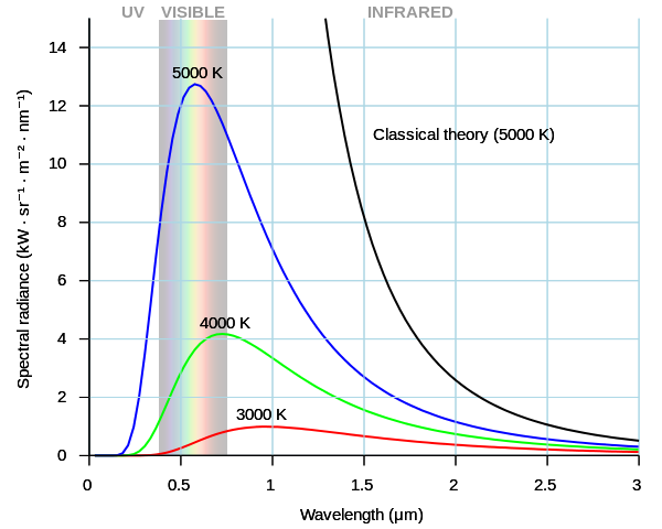
The temperature corresponding to the blue curve is higher than the temperature corresponding to the red curve. Since \(\lambda =c/\nu\), we can also use the frequency \(\nu\) to characterize the radiation spectrum.

Classical mechanics predicts that the intensity \(I\) of emitted radiation at frequency \(\nu\) is given by

\[I(\nu)=\dfrac{8\pi k_B T \nu^2}{c^3} \label{4.5}\]

where \(k_B\) is Boltzmann's constant, \(k_B=1.38066*10^{-23} \ J/K\). The classical curves in the above figure are obtained by setting \(\nu =c/\lambda\) in this expression:

\[I(\lambda )=\dfrac{8\pi k_B T}{c\lambda^2} \label{4.6}\]

and are shown as the dashed curves in the figure. Note that as \(\lambda \rightarrow 0\), \(I \rightarrow \infty\), which is known as the ultraviolet catastrophe.

In the classical theory, blackbody radiation is modeled as the radiation emitted from oscillating charged particles at the object's surface. These oscillations are produced by the thermal motions of the charged particles. If we treat each particle as a simple harmonic oscillator, then we can easily understand how Planck was able to explain blackbody radiation.

A simple harmonic oscillator is described by a Hooke's law force

\[F=-k(x-x_0 ) \label{4.7}\]

where the force \(F\) arises from the displacement \(x\) from the equilibrium position \(x_0\) of a charged particle attached to a spring. Here \(k\) is the spring constant, which measures the stiffness of the spring.

Figure 7:

The force \(F\) is derived from the potential energy curve

\[V(x)=\dfrac{1}{2}k(x-x_0)^2\]

and produces the following motion in \(x\):

\[x(t)=x_0 +Acos(2\pi \nu t+\phi)\]

where

\[\nu =\dfrac{1}{2\pi }\sqrt{\dfrac{k}{m}}\]

and \(\phi\) is known as the phase angle. Its value is determined by the initial position \(x(0)\) and initial momentum \(p(0)\) of the oscillator. The energy \[E=\dfrac{p^2}{2m}+\dfrac{1}{2}k(x-x_0 )^2\] can take on any value, as determined by the initial conditions, but once its value is set, it does not change over time because energy is conserved.

Planck's ingenious idea was to propose the following radical hypothesis: What if the energy \(E\) could not take on just any value but only certain discrete values called "quanta" of energy. He suggested that higher frequency motion meant higher energy. By the way, in classical mechanics, the energy is only determined by the amplitude of the oscillator, not the frequency. Thus, he proposed that the energy quanta be multiplies of the frequency

\[E\propto n\nu\]

where \(n\) is an integer \(n=0,1,2,...\). The constant of proportionality needed to give energy units he called \(h\), which is now known as Planck's constant. Thus, the discrete energy values were proposed to be determined by

\[E=nh\nu\]

Since there are many oscillating charged particles, we need to consider a very large number of identical oscillating systems. At Planck's time, it was known that the probability that a collection of identical systems at the same temperature \(T\) but starting from different classical initial conditions would have an energy \(E\) was proportional to the Boltzmann factor

\[probability \propto e^{-E/k_B T}\]

Let us recall the definition of a probability. Generally, given \(N\) possible events \(\epsilon_1 ,...,\epsilon_N\), the probability that an event \(\epsilon_n\) will occur is defined to be

\[probability \ that \ \epsilon_n \ occurs\equiv P(\epsilon_n)=\dfrac{Number \ of \ ways \ \epsilon_n \ can \ occur}{Total \ number \ of \ ways \ any \ event \ can \ occur}\]

Planck applied this formula to his quantized energy values. Let the event \(\epsilon_n\) be a measurement of the energy of the system at temperature \(T\) that yields an energy \(E=nh\nu\). The probability of such an event, according to the above formula is

\[probability=\dfrac{e^{-nh\nu /k_B T}}{\sum_{n=0}^{\infty}e^{-nh\nu /k_B T}}\]

Note that if we sum both sides over \(n\), we must get 1. That is, the sum over \(n\) is the probability of finding the system with any allowable energy, which, of course, must be 1. The denominator is of the form

\[\sum_{n=0}^{\infty}\left ( e^{-h\nu /k_B T} \right )^n\]

and since \(0< exp(-h\nu /k_B T)<1\), it follows that the sum is nothing more than a geometric series for which the following summation formula applies

\[\sum_{n=0}^{\infty}r^n =\dfrac{1}{1-r}\]

where \(0<r<1\). Applying this to the probability formula, we obtain

\[probability=e^{-nh\nu /k_B T}(1-e^{-h\nu /k_B T})\]

Similarly, the average energy of such a collection of systems is

\[\bar{E}=\dfrac{\sum_{n=0}^{\infty}nh\nu e^{-nh\nu /k_B T}}{\sum_{n=0}^{\infty}e^{-nh\nu /k_B T}}\]

These sums can be worked out (with a lot of algebra not presented here) with the result

\[\bar{E}=\dfrac{h\nu}{e^{h\nu /k_B T}-1}\]

From this average energy formula, Planck was able to show that the intensity of emitted radiation from the blackbody would be given by

\[I(\nu )=\dfrac{8\pi h\nu^3}{c^3}\dfrac{1}{e^{h\nu /k_B T}-1}\]

or using \(\nu =c/\lambda\)

\[I(\lambda )=\dfrac{8\pi h}{\lambda^3}\dfrac{1}{e^{hc/\lambda k_B T}-1}\]

Plotting this curve as a function of \(\lambda\) yields the solid lines in the radiation spectra shown above.

By fitting this expression to the experimental data, he was able to determine a value for \(h\), which is now accepted to be \(h=6.6208*10^{-34} \ J\cdot s\). Planck's formula actually reduces to the classical formula in the limit that the difference between successive quantized energy values \(\Delta E=h\nu\) is small compared to \(k_B T\), i.e.

\[\dfrac{h\nu}{k_B T}\ll 1\]

When this is true, the exponential can be approximated using the formula \(e^x \approx 1+x\), so that

\[e^{h\nu /k_B T}\approx 1+\dfrac{h\nu}{k_B T}\]

In this case

\[\begin{align*}I(\nu ) &\rightarrow \dfrac{8\pi h\nu^3}{c^3}\dfrac{1}{1+h\nu /k_B T-1}\\ &= \dfrac{8\pi h\nu^3}{c^3}\dfrac{k_B T}{h\nu}\\ &= \dfrac{8\pi k_B T\nu^2}{c^3}\end{align*}\]

Planck's proposed theory about energy quantization was able to explain the blackbody radiation spectra, yet it constituted a radical departure from classical physics.

The Photoelectric Effect

The photoelectric effect was explained by Albert Einstein in 1905. When light impinges on a metal surface, it is observed that for sufficiently high frequency light, electrons will be ejected from the surface as shown in the figure below:

Figure 8:

Classical theory predicts that energy carried by light is proportional to its amplitude independent of its frequency, and this fails to correctly explain the experiment.

Einstein, borrowing Planck's hypothesis about the quantized energy of an oscillator, suggested that light comes in packets or "quanta" with energy \(E\) given by Planck's formula with \(n=1\)

\[E=h\nu\]

Since, according to both Planck and Einstein, the energy of light is proportional to its frequency rather than its amplitude, there will be a minimum frequency \(\nu_0\) needed to eject an electron with no residual energy. The corresponding energy is

\[h\nu_0 =\Phi\]\

where \(\Phi\) is called the work function of the metal, and it is an intrinsic property of the metal. In general, if \(\nu >\nu_0\), an electron will be ejected with some residual kinetic energy. If the electron has momentum \(p\) leaving the surface, then this kinetic energy is \(p^2 /2m_e\), and because energy is conserved, we have the relation

\[h\nu =\Phi +\dfrac{p^2}{2m_e}\]

The left side is the energy of the impinging light, and the right side if the sum of the minimum energy needed to extract an electron and the residual kinetic energy it has when leaving the surface.

The strange implication of this experiment is that light can behave as a kind of massless "particle" now known as a photon whose energy \(E=h\nu\) can be transferred to an actual particle (an electron), imparting kinetic energy to it, just as in an elastic collision between to massive particles such as billiard balls

Contributors and Attributions

• Mark Tuckerman (New York University)

• Michael Fowler (Beams Professor, Department of Physics, University of Virginia)