1.4: The Kinetic Molecular Theory of Gases

Theoretical models attempting to describe the nature of gases date back to the earliest scientific inquiries into the nature of matter and even earlier! In about 50 BC, Lucretius, a Roman philosopher, proposed that macroscopic bodies were composed of atoms that continually collide with one another and are in constant motion, despite the observable reality that the body itself is as rest. However, Lucretius’ ideas went largely ignored as they deviated from those of Aristotle, whose views were more widely accepted at the time.

In 1738, Daniel Bernoulli (Bernoulli, 1738) published a model that contains the basic framework for the modern Kinetic Molecular theory. Rudolf Clausius furthered the model in 1857 by (among other things) introducing the concept of mean free path (Clausius, 1857). These ideas were further developed by Maxwell (Maxwell, Molecules, 1873). But, because atomic theory was not fully embraced in the early 20^th century, it was not until Albert Einstein published one of his seminal works describing Brownian motion (Einstein, 1905) in which he modeled matter using a kinetic theory of molecules that the idea of an atomic (or molecular) picture really took hold in the scientific community.

In its modern form, the Kinetic Molecular Theory of gasses is based on five basic postulates.

1. Gas particles obey Newton’s laws of motion and travel in straight lines unless they collide with other particles or the walls of the container.
2. Gas particles are very small compared to the averages of the distances between them.
3. Molecular collisions are perfectly elastic so that kinetic energy is conserved.
4. Gas particles so not interact with other particles except through collisions. There are no attractive or repulsive forces between particles.
5. The average kinetic energy of the particles in a sample of gas is proportional to the temperature.

Qualitatively, this model predicts the form of the ideal gas law.

1. More particles means more collisions with the wall \[ p \propto n \]
2. Smaller volume means more frequent collisions with the wall \[ p \propto \dfrac{1}{V} \]
3. Higher molecular speeds means more frequent collisions with the walls \[ p \propto n \]

Putting all of these together yields

\[ p \propto \dfrac{nT}{V} =k \dfrac{nT}{V}\]

which is exactly the form of the ideal gas law! The remainder of the job is to derive a value for the constant of proportionality (\(k\)) that is consistent with experimental observation.

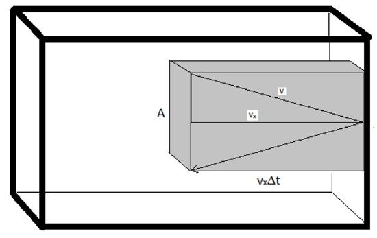
For simplicity, imagine a collection of gas particles in a fixed-volume container with all of the particles traveling at the same velocity. What implications would the kinetic molecular theory have on such a sample? One approach to answering this question is to derive an expression for the pressure of the gas.

The pressure is going to be determined by considering the collisions of gas molecules with the wall of the container. Each collision will impart some force. So the greater the number of collisions, the greater the pressure will be. Also, the larger force imparted per collision, the greater the pressure will be. And finally, the larger the area over which collisions are spread, the smaller the pressure will be.

\[ p \propto \dfrac{ (\text{number of collisions}) \times (\text{force imparted per collision})}{area}\]

Figure \(\PageIndex{1}\): The "collision volume" is the subset of the total volume that contains molecules that will actually collide with area \(A\) in the time interval \(\Delta t\).

We can use a Maxwell-Boltzmann distribution to determine the average velocities the molecules are traveling at which allows us to determine how much force they hit the wall with and how often the molecules hit the wall.