
9.3: The Total Differential
- Page ID
- 238250

\( \newcommand{\vecs}[1]{\overset { \scriptstyle \rightharpoonup} {\mathbf{#1}} } \)
\( \newcommand{\vecd}[1]{\overset{-\!-\!\rightharpoonup}{\vphantom{a}\smash {#1}}} \)
\( \newcommand{\dsum}{\displaystyle\sum\limits} \)
\( \newcommand{\dint}{\displaystyle\int\limits} \)
\( \newcommand{\dlim}{\displaystyle\lim\limits} \)
\( \newcommand{\id}{\mathrm{id}}\) \( \newcommand{\Span}{\mathrm{span}}\)
( \newcommand{\kernel}{\mathrm{null}\,}\) \( \newcommand{\range}{\mathrm{range}\,}\)
\( \newcommand{\RealPart}{\mathrm{Re}}\) \( \newcommand{\ImaginaryPart}{\mathrm{Im}}\)
\( \newcommand{\Argument}{\mathrm{Arg}}\) \( \newcommand{\norm}[1]{\| #1 \|}\)
\( \newcommand{\inner}[2]{\langle #1, #2 \rangle}\)
\( \newcommand{\Span}{\mathrm{span}}\)
\( \newcommand{\id}{\mathrm{id}}\)
\( \newcommand{\Span}{\mathrm{span}}\)
\( \newcommand{\kernel}{\mathrm{null}\,}\)
\( \newcommand{\range}{\mathrm{range}\,}\)
\( \newcommand{\RealPart}{\mathrm{Re}}\)
\( \newcommand{\ImaginaryPart}{\mathrm{Im}}\)
\( \newcommand{\Argument}{\mathrm{Arg}}\)
\( \newcommand{\norm}[1]{\| #1 \|}\)
\( \newcommand{\inner}[2]{\langle #1, #2 \rangle}\)
\( \newcommand{\Span}{\mathrm{span}}\) \( \newcommand{\AA}{\unicode[.8,0]{x212B}}\)
\( \newcommand{\vectorA}[1]{\vec{#1}} % arrow\)
\( \newcommand{\vectorAt}[1]{\vec{\text{#1}}} % arrow\)
\( \newcommand{\vectorB}[1]{\overset { \scriptstyle \rightharpoonup} {\mathbf{#1}} } \)
\( \newcommand{\vectorC}[1]{\textbf{#1}} \)
\( \newcommand{\vectorD}[1]{\overrightarrow{#1}} \)
\( \newcommand{\vectorDt}[1]{\overrightarrow{\text{#1}}} \)
\( \newcommand{\vectE}[1]{\overset{-\!-\!\rightharpoonup}{\vphantom{a}\smash{\mathbf {#1}}}} \)
\( \newcommand{\vecs}[1]{\overset { \scriptstyle \rightharpoonup} {\mathbf{#1}} } \)
\(\newcommand{\longvect}{\overrightarrow}\)
\( \newcommand{\vecd}[1]{\overset{-\!-\!\rightharpoonup}{\vphantom{a}\smash {#1}}} \)
\(\newcommand{\avec}{\mathbf a}\) \(\newcommand{\bvec}{\mathbf b}\) \(\newcommand{\cvec}{\mathbf c}\) \(\newcommand{\dvec}{\mathbf d}\) \(\newcommand{\dtil}{\widetilde{\mathbf d}}\) \(\newcommand{\evec}{\mathbf e}\) \(\newcommand{\fvec}{\mathbf f}\) \(\newcommand{\nvec}{\mathbf n}\) \(\newcommand{\pvec}{\mathbf p}\) \(\newcommand{\qvec}{\mathbf q}\) \(\newcommand{\svec}{\mathbf s}\) \(\newcommand{\tvec}{\mathbf t}\) \(\newcommand{\uvec}{\mathbf u}\) \(\newcommand{\vvec}{\mathbf v}\) \(\newcommand{\wvec}{\mathbf w}\) \(\newcommand{\xvec}{\mathbf x}\) \(\newcommand{\yvec}{\mathbf y}\) \(\newcommand{\zvec}{\mathbf z}\) \(\newcommand{\rvec}{\mathbf r}\) \(\newcommand{\mvec}{\mathbf m}\) \(\newcommand{\zerovec}{\mathbf 0}\) \(\newcommand{\onevec}{\mathbf 1}\) \(\newcommand{\real}{\mathbb R}\) \(\newcommand{\twovec}[2]{\left[\begin{array}{r}#1 \\ #2 \end{array}\right]}\) \(\newcommand{\ctwovec}[2]{\left[\begin{array}{c}#1 \\ #2 \end{array}\right]}\) \(\newcommand{\threevec}[3]{\left[\begin{array}{r}#1 \\ #2 \\ #3 \end{array}\right]}\) \(\newcommand{\cthreevec}[3]{\left[\begin{array}{c}#1 \\ #2 \\ #3 \end{array}\right]}\) \(\newcommand{\fourvec}[4]{\left[\begin{array}{r}#1 \\ #2 \\ #3 \\ #4 \end{array}\right]}\) \(\newcommand{\cfourvec}[4]{\left[\begin{array}{c}#1 \\ #2 \\ #3 \\ #4 \end{array}\right]}\) \(\newcommand{\fivevec}[5]{\left[\begin{array}{r}#1 \\ #2 \\ #3 \\ #4 \\ #5 \\ \end{array}\right]}\) \(\newcommand{\cfivevec}[5]{\left[\begin{array}{c}#1 \\ #2 \\ #3 \\ #4 \\ #5 \\ \end{array}\right]}\) \(\newcommand{\mattwo}[4]{\left[\begin{array}{rr}#1 \amp #2 \\ #3 \amp #4 \\ \end{array}\right]}\) \(\newcommand{\laspan}[1]{\text{Span}\{#1\}}\) \(\newcommand{\bcal}{\cal B}\) \(\newcommand{\ccal}{\cal C}\) \(\newcommand{\scal}{\cal S}\) \(\newcommand{\wcal}{\cal W}\) \(\newcommand{\ecal}{\cal E}\) \(\newcommand{\coords}[2]{\left\{#1\right\}_{#2}}\) \(\newcommand{\gray}[1]{\color{gray}{#1}}\) \(\newcommand{\lgray}[1]{\color{lightgray}{#1}}\) \(\newcommand{\rank}{\operatorname{rank}}\) \(\newcommand{\row}{\text{Row}}\) \(\newcommand{\col}{\text{Col}}\) \(\renewcommand{\row}{\text{Row}}\) \(\newcommand{\nul}{\text{Nul}}\) \(\newcommand{\var}{\text{Var}}\) \(\newcommand{\corr}{\text{corr}}\) \(\newcommand{\len}[1]{\left|#1\right|}\) \(\newcommand{\bbar}{\overline{\bvec}}\) \(\newcommand{\bhat}{\widehat{\bvec}}\) \(\newcommand{\bperp}{\bvec^\perp}\) \(\newcommand{\xhat}{\widehat{\xvec}}\) \(\newcommand{\vhat}{\widehat{\vvec}}\) \(\newcommand{\uhat}{\widehat{\uvec}}\) \(\newcommand{\what}{\widehat{\wvec}}\) \(\newcommand{\Sighat}{\widehat{\Sigma}}\) \(\newcommand{\lt}{<}\) \(\newcommand{\gt}{>}\) \(\newcommand{\amp}{&}\) \(\definecolor{fillinmathshade}{gray}{0.9}\)In Chapter 8 we learned that partial derivatives indicate how the dependent variable changes with one particular independent variable keeping the others fixed. In the context of an equation of state \(P=P(T,V,n)\), the partial derivative of \(P\) with respect to \(V\) at constant \(T\) and \(n\) is:
\[\left (\dfrac{\partial P}{\partial V} \right )_{T,n} \nonumber \]
and physically represents how the pressure varies as we change the volume at constant temperature and constant \(n\).
The partial derivative of \(P\) with respect to \(T\) at constant \(V\) and \(n\) is:
\[\left (\dfrac{\partial P}{\partial T} \right )_{V,n} \nonumber \]
and physically represents how the pressure varies as we change the temperature at constant volume and constant \(n\).
What happens with the dependent variable (in this case \(P\)) if we change two or more independent variables simultaneously? For an infinitesimal change in volume and temperature, we can write the change in pressure as:
\[\label{eq:differentials1} dP=\left (\dfrac{\partial P}{\partial V} \right )_{T,n} dV+\left (\dfrac{\partial P}{\partial T} \right )_{V,n} dT \]
Equation \ref{eq:differentials1} is called the total differential of P, and it simply states that the change in \(P\) is the sum of the individual contributions due to the change in \(V\) at constant \(T\) and the change in \(T\) at constant \(V\). This equation is true for infinitesimal changes. If the changes are not infinitesimal we will integrate this expression to calculate the change in \(P\).[differentials_position1]
Let’s now consider the volume of a fluid, which is a function of pressure, temperature and the number of moles: \(V=V(n,T,P)\). The total differential of \(V\), by definition, is:
\[\label{eq:differentials3} dV=\left (\frac{\partial V}{\partial T} \right )_{P,n} dT+\left (\frac{\partial V}{\partial P} \right )_{T,n} dP+\left (\frac{\partial V}{\partial n} \right )_{T,V} dn \]
If we want to calculate the change in volume in a fluid upon small changes in \(P, T\) and \(n\), we could use:
\[\label{eq:differentials3b} \Delta V\approx \left (\frac{\partial V}{\partial T} \right )_{P,n} \Delta T+\left (\frac{\partial V}{\partial P} \right )_{T,n} \Delta P+\left (\frac{\partial V}{\partial n} \right )_{T,V} \Delta n \]
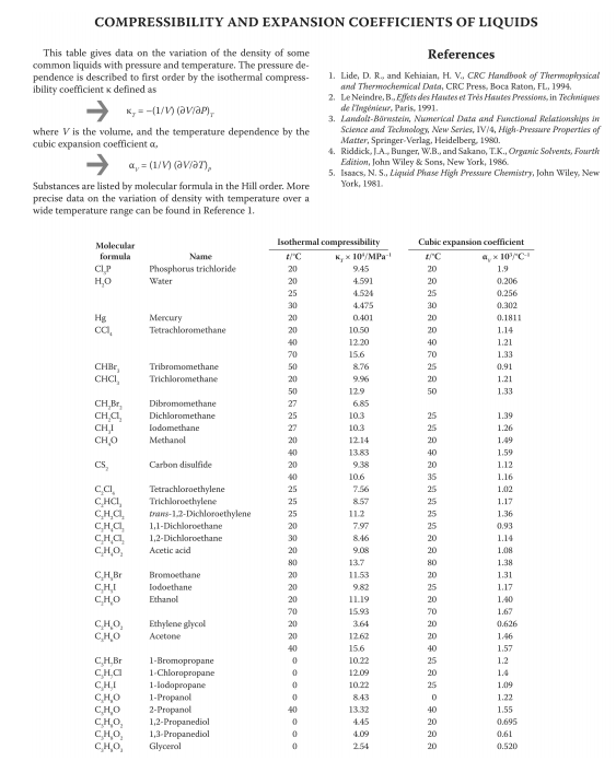
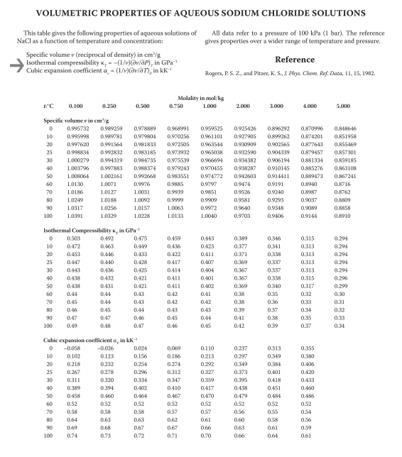
Of course, if we know the function \(V=V(n,T,P)\), we could also calculate \(\Delta V\) as \(V_f-F_i\), where the final and initial volumes are calculated using the final and initial values of \(P, T\) and \(n\). This seems easy, so why do we need to bother with Equation \ref{eq:differentials3b}? The reason is that sometimes we can measure the partial derivatives experimentally, but we do not have an equation of the type \(V=V(n,T,P)\) to use. For example, the following quantities are accessible experimentally and tabulated for different fluids and materials (Fig. [fig:diff_tables]):
- \(\alpha=\frac{1}{V}\left(\frac{\partial V}{\partial T} \right )_{P,n}\) (coefficient of thermal expansion)
- \(\kappa=-\frac{1}{V}\left(\frac{\partial V}{\partial P} \right )_{V,n}\) (isothermal compressibility)[differentials:compressibility]
- \(V_m=\left(\frac{\partial V}{\partial n} \right )_{P,T}\) (molar volume)
Using these definitions, Equation \ref{eq:differentials3} becomes:
\[\label{eq:differentials4} dV=\alpha V dT-\kappa VdP+V_m dn \]
You can find tables with experimentally determined values of \(\alpha\) and \(\kappa\) under different conditions, which you can use to calculate the changes in \(V\). Again, as we will see later in this chapter, this equation will need to be integrated if the changes are not small. In any case, the point is that you may have access to information about the derivatives of the function, but not to the function itself (in this case \(V\) as a function of \(T, P, n\)).
In general, for a function \(u=u(x_1, x_2...x_n)\), we define the total differential of \(u\) as:
\[\label{eq:total_differential} du=\left (\frac{\partial u}{\partial x_1} \right )_{x_2...x_n} dx_1+\left (\frac{\partial u}{\partial x_2} \right )_{x_1, x_3...x_n} dx_2+...+\left (\frac{\partial u}{\partial x_n} \right )_{x_1...x_{n-1}} dx_n \]
Calculate the total differential of the function \(z=3x^3+3yx^2+xy^2\).
Solution
By definition, the total differential is:
\[dz=\left (\frac{\partial z}{\partial x} \right )_{y} dx+\left (\frac{\partial z}{\partial y} \right )_{x} dy \nonumber \]
For the function given in the problem,
\[\left (\frac{\partial z}{\partial x} \right )_{y}=9x^2+6xy+y^2 \nonumber \]
and
\[\left (\frac{\partial z}{\partial y} \right )_{x}=3x^2+2xy \nonumber \]
and therefore,
\[\displaystyle{\color{Maroon}dz=(9x^2+6xy+y^2)dx+(3x^2+2xy)dy} \nonumber \]
Want to see more examples?
- Example 1: http://www.youtube.com/watch?v=z0TxZ0EHzIg Notice that she calls it ’the differential’, but I prefer ’the total differential’.