
11.5: Hypothesis Test for a Population Mean (3 of 5)
- Page ID
- 251446
\( \newcommand{\vecs}[1]{\overset { \scriptstyle \rightharpoonup} {\mathbf{#1}} } \)
\( \newcommand{\vecd}[1]{\overset{-\!-\!\rightharpoonup}{\vphantom{a}\smash {#1}}} \)
\( \newcommand{\id}{\mathrm{id}}\) \( \newcommand{\Span}{\mathrm{span}}\)
( \newcommand{\kernel}{\mathrm{null}\,}\) \( \newcommand{\range}{\mathrm{range}\,}\)
\( \newcommand{\RealPart}{\mathrm{Re}}\) \( \newcommand{\ImaginaryPart}{\mathrm{Im}}\)
\( \newcommand{\Argument}{\mathrm{Arg}}\) \( \newcommand{\norm}[1]{\| #1 \|}\)
\( \newcommand{\inner}[2]{\langle #1, #2 \rangle}\)
\( \newcommand{\Span}{\mathrm{span}}\)
\( \newcommand{\id}{\mathrm{id}}\)
\( \newcommand{\Span}{\mathrm{span}}\)
\( \newcommand{\kernel}{\mathrm{null}\,}\)
\( \newcommand{\range}{\mathrm{range}\,}\)
\( \newcommand{\RealPart}{\mathrm{Re}}\)
\( \newcommand{\ImaginaryPart}{\mathrm{Im}}\)
\( \newcommand{\Argument}{\mathrm{Arg}}\)
\( \newcommand{\norm}[1]{\| #1 \|}\)
\( \newcommand{\inner}[2]{\langle #1, #2 \rangle}\)
\( \newcommand{\Span}{\mathrm{span}}\) \( \newcommand{\AA}{\unicode[.8,0]{x212B}}\)
\( \newcommand{\vectorA}[1]{\vec{#1}} % arrow\)
\( \newcommand{\vectorAt}[1]{\vec{\text{#1}}} % arrow\)
\( \newcommand{\vectorB}[1]{\overset { \scriptstyle \rightharpoonup} {\mathbf{#1}} } \)
\( \newcommand{\vectorC}[1]{\textbf{#1}} \)
\( \newcommand{\vectorD}[1]{\overrightarrow{#1}} \)
\( \newcommand{\vectorDt}[1]{\overrightarrow{\text{#1}}} \)
\( \newcommand{\vectE}[1]{\overset{-\!-\!\rightharpoonup}{\vphantom{a}\smash{\mathbf {#1}}}} \)
\( \newcommand{\vecs}[1]{\overset { \scriptstyle \rightharpoonup} {\mathbf{#1}} } \)
\( \newcommand{\vecd}[1]{\overset{-\!-\!\rightharpoonup}{\vphantom{a}\smash {#1}}} \)
\(\newcommand{\avec}{\mathbf a}\) \(\newcommand{\bvec}{\mathbf b}\) \(\newcommand{\cvec}{\mathbf c}\) \(\newcommand{\dvec}{\mathbf d}\) \(\newcommand{\dtil}{\widetilde{\mathbf d}}\) \(\newcommand{\evec}{\mathbf e}\) \(\newcommand{\fvec}{\mathbf f}\) \(\newcommand{\nvec}{\mathbf n}\) \(\newcommand{\pvec}{\mathbf p}\) \(\newcommand{\qvec}{\mathbf q}\) \(\newcommand{\svec}{\mathbf s}\) \(\newcommand{\tvec}{\mathbf t}\) \(\newcommand{\uvec}{\mathbf u}\) \(\newcommand{\vvec}{\mathbf v}\) \(\newcommand{\wvec}{\mathbf w}\) \(\newcommand{\xvec}{\mathbf x}\) \(\newcommand{\yvec}{\mathbf y}\) \(\newcommand{\zvec}{\mathbf z}\) \(\newcommand{\rvec}{\mathbf r}\) \(\newcommand{\mvec}{\mathbf m}\) \(\newcommand{\zerovec}{\mathbf 0}\) \(\newcommand{\onevec}{\mathbf 1}\) \(\newcommand{\real}{\mathbb R}\) \(\newcommand{\twovec}[2]{\left[\begin{array}{r}#1 \\ #2 \end{array}\right]}\) \(\newcommand{\ctwovec}[2]{\left[\begin{array}{c}#1 \\ #2 \end{array}\right]}\) \(\newcommand{\threevec}[3]{\left[\begin{array}{r}#1 \\ #2 \\ #3 \end{array}\right]}\) \(\newcommand{\cthreevec}[3]{\left[\begin{array}{c}#1 \\ #2 \\ #3 \end{array}\right]}\) \(\newcommand{\fourvec}[4]{\left[\begin{array}{r}#1 \\ #2 \\ #3 \\ #4 \end{array}\right]}\) \(\newcommand{\cfourvec}[4]{\left[\begin{array}{c}#1 \\ #2 \\ #3 \\ #4 \end{array}\right]}\) \(\newcommand{\fivevec}[5]{\left[\begin{array}{r}#1 \\ #2 \\ #3 \\ #4 \\ #5 \\ \end{array}\right]}\) \(\newcommand{\cfivevec}[5]{\left[\begin{array}{c}#1 \\ #2 \\ #3 \\ #4 \\ #5 \\ \end{array}\right]}\) \(\newcommand{\mattwo}[4]{\left[\begin{array}{rr}#1 \amp #2 \\ #3 \amp #4 \\ \end{array}\right]}\) \(\newcommand{\laspan}[1]{\text{Span}\{#1\}}\) \(\newcommand{\bcal}{\cal B}\) \(\newcommand{\ccal}{\cal C}\) \(\newcommand{\scal}{\cal S}\) \(\newcommand{\wcal}{\cal W}\) \(\newcommand{\ecal}{\cal E}\) \(\newcommand{\coords}[2]{\left\{#1\right\}_{#2}}\) \(\newcommand{\gray}[1]{\color{gray}{#1}}\) \(\newcommand{\lgray}[1]{\color{lightgray}{#1}}\) \(\newcommand{\rank}{\operatorname{rank}}\) \(\newcommand{\row}{\text{Row}}\) \(\newcommand{\col}{\text{Col}}\) \(\renewcommand{\row}{\text{Row}}\) \(\newcommand{\nul}{\text{Nul}}\) \(\newcommand{\var}{\text{Var}}\) \(\newcommand{\corr}{\text{corr}}\) \(\newcommand{\len}[1]{\left|#1\right|}\) \(\newcommand{\bbar}{\overline{\bvec}}\) \(\newcommand{\bhat}{\widehat{\bvec}}\) \(\newcommand{\bperp}{\bvec^\perp}\) \(\newcommand{\xhat}{\widehat{\xvec}}\) \(\newcommand{\vhat}{\widehat{\vvec}}\) \(\newcommand{\uhat}{\widehat{\uvec}}\) \(\newcommand{\what}{\widehat{\wvec}}\) \(\newcommand{\Sighat}{\widehat{\Sigma}}\) \(\newcommand{\lt}{<}\) \(\newcommand{\gt}{>}\) \(\newcommand{\amp}{&}\) \(\definecolor{fillinmathshade}{gray}{0.9}\)
Learning Objectives
- Under appropriate conditions, conduct a hypothesis test about a mean for a matched pairs design. State a conclusion in context.
Another common use of the t-test for a population mean is in “before and after” situations. In this situation, we have two quantitative measurements from a single sample of individuals. This is an example of a matched-pairs design.
Example
Drinking and Driving
The Centers for Disease Control and Prevention (CDC) website cites studies from the National Highway Traffic Safety Administration to support this statement: “Alcohol use slows reaction time and impairs judgment and coordination, which are all skills needed to drive a car safely. The more alcohol consumed, the greater the impairment.” All states in the United States have adopted a blood alcohol concentration of 0.08% (80 mg/dL) as the legal limit for operating a motor vehicle. The CDC website continues, “Note: Legal limits do not define a level below which it is safe to operate a vehicle or engage in some other activity. Impairment due to alcohol use begins to occur at levels well below the legal limit.”
It is this last statement that may be surprising to drivers. Interviews with drunk drivers who were involved in accidents reveal that drunk drivers do not realize how drunk they are. “I only had one or two drinks – I am okay to drive” is a common sentiment. Suppose a college conducts a study to call attention to this issue. Researchers use a random sample of 20 college students to examine the effect of drinking two beers on reaction times. They use a driving simulator to measure each student’s reaction time before and after drinking two beers. The reaction time is the time it takes the student to hit the brakes in the simulator when an obstacle appears in the road.
In this situation, we have two quantitative measurements for each student. To measure the effect of the two beers, we subtract the two reaction times to create one measurement of “change” or “effect.” This controls the effects of individual characteristics that could influence reaction time, such as driving experience or natural quickness.
Here is a partial list of the data. We define the difference as “before minus after.” If the “after” reaction time is longer, then the difference is negative. A negative value means the reaction time is slower after drinking.
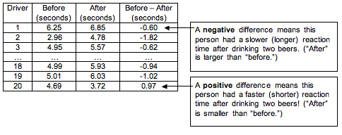
Note: It is common to define the difference in measurements as “before minus after.” But we could also define the difference the other way around as “after minus before.” In this definition, if the “after” reaction time is longer, then the difference is positive, so a slower reaction time after drinking corresponds to a positive value. This makes less intuitive sense to us. We want “negative” to mean “drinking has a negative effect,” so we used the other definition, “before minus after.”
Step 1: Determine the hypotheses.
The null hypothesis is a claim of “no change” or “no effect.” The alternative hypothesis reflects the claim.
- H0: Drinking two beers has no effect on reaction time.
- Ha: Drinking two beers slows reaction time.
If drinking two beers has no effect on reaction time, then the mean of the differences in reaction times (before minus after) will be zero. If drinking two beers slows reaction time, then the mean of the differences in reaction times (before minus after) will be negative. So we can rewrite our hypotheses as follows.
- H0: μ = 0
- Ha: μ < 0
where µ is the mean of the difference in reaction time (before minus after) for all students at this college after drinking two beers.
Suppose researchers set a significance level of 5%.
Note: if we defined the difference in reverse order as “after minus before,” then a positive difference corresponds to a slower reaction time. This changes the alternative hypothesis to Ha: µ > 0. This will not effect the P-value or our conclusion. You just have to make sure the alternative hypothesis says what you want it to say given the way you define the difference.
Note: In some textbooks and other statistical materials, you will see the “mean of the difference” written as μd.
Step 2: Collect the data.
Here is the (made-up) data from this sample of 20 college students. The mean of the differences (before minus after) is approximately −0.46 seconds, and the standard deviation is approximately 0.87 seconds.
Step 3: Assess the evidence.
Check the Criteria for Use of a T-Model
The sample size is only 20, and we do not know if these differences would be normally distributed in general when comparing these two treatments in the population of all college students. We therefore do not meet the conditions for use of a t-model. Some researchers would stop here and not complete the hypothesis test. Others would check the shape of the distribution of differences in the sample. If the sample is approximately normal (or at least not heavily skewed), then they view this as a hopeful indication that the distribution in the population will also be approximately normal, and they continue with the hypothesis test, adding a disclaimer to the conclusion.
Here is a histogram of the differences in the sample.
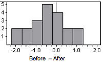
The data is not heavily skewed, so we are willing to proceed with the t-test.
Compute the Test Statistic
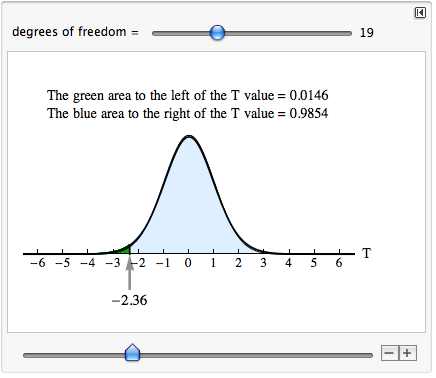
Find the P-value.
We use the simulation with the t-model for 19 degrees of freedom (df = n − 1 = 20 − 1 = 19). The P-value is approximately 0.015.
Step 4: State a conclusion.
The P-value (0.015) is less than the significance level (0.05), so we reject the null and accept the alternative hypothesis that µ < 0.
This study suggests that reactions times when driving are significantly slower after drinking two beers for students at this college. (P = 0.015).
It is good practice to include a disclaimer with this conclusion because the sample is small. We might add the following to our conclusion if we were publicly presenting these results: “The sample was too small to formally met the requirements for a t-test. On the basis of the data, we are assuming that the difference in reaction times would be normally distributed in general when comparing these two treatments in the population of all college students. The conclusion from this test is valid only if this assumption is true.”
Comment
From this study, can we generalize to a larger population of “all college students” or “all drivers”? Technically, such a generalization requires that the sample be randomly selected from the more general population. Is this type of random sampling done in practice? Not always. The matched pairs design controls for individual differences that would otherwise confound such a generalization. This is one of the reasons that researchers run hypothesis tests with data gathered by groups like the National Highway Traffic Safety Administration, even when participants are not randomly selected. But ideally we should select samples randomly from the population of interest.
Can we make a cause-and-effect conclusion from this study?
We should be cautious about a cause-and-effect conclusion here because there is no random assignment. We take measurements from every student in both the treatment and the control setting without randomizing the treatment order. Every participant did the driving test sober, then drank two beers and did the driving test again. Technically, we need a more sophisticated study design that uses random assignment in order to make cause-and-effect conclusions. For example, we could randomly assign the treatment order for each student by flipping a coin, assigning some students do the first driving test while sober and others do the first driving test after drinking two beers. Then everyone comes back on another day to complete the part of the experiment that he or she had not done.
The following activities give you an opportunity to practice parts of the hypothesis testing process. In each of these activities, the study is a matched-pairs design, so the population mean represents a mean of differences in paired measurements. Later you will have the opportunity to practice the hypothesis test from start to finish.
Learn By Doing
Learn By Doing
- Concepts in Statistics. Provided by: Open Learning Initiative. Located at: http://oli.cmu.edu. License: CC BY: Attribution