
9.2: Hypothesis Testing (5 of 5)
- Page ID
- 251405
\( \newcommand{\vecs}[1]{\overset { \scriptstyle \rightharpoonup} {\mathbf{#1}} } \)
\( \newcommand{\vecd}[1]{\overset{-\!-\!\rightharpoonup}{\vphantom{a}\smash {#1}}} \)
\( \newcommand{\id}{\mathrm{id}}\) \( \newcommand{\Span}{\mathrm{span}}\)
( \newcommand{\kernel}{\mathrm{null}\,}\) \( \newcommand{\range}{\mathrm{range}\,}\)
\( \newcommand{\RealPart}{\mathrm{Re}}\) \( \newcommand{\ImaginaryPart}{\mathrm{Im}}\)
\( \newcommand{\Argument}{\mathrm{Arg}}\) \( \newcommand{\norm}[1]{\| #1 \|}\)
\( \newcommand{\inner}[2]{\langle #1, #2 \rangle}\)
\( \newcommand{\Span}{\mathrm{span}}\)
\( \newcommand{\id}{\mathrm{id}}\)
\( \newcommand{\Span}{\mathrm{span}}\)
\( \newcommand{\kernel}{\mathrm{null}\,}\)
\( \newcommand{\range}{\mathrm{range}\,}\)
\( \newcommand{\RealPart}{\mathrm{Re}}\)
\( \newcommand{\ImaginaryPart}{\mathrm{Im}}\)
\( \newcommand{\Argument}{\mathrm{Arg}}\)
\( \newcommand{\norm}[1]{\| #1 \|}\)
\( \newcommand{\inner}[2]{\langle #1, #2 \rangle}\)
\( \newcommand{\Span}{\mathrm{span}}\) \( \newcommand{\AA}{\unicode[.8,0]{x212B}}\)
\( \newcommand{\vectorA}[1]{\vec{#1}} % arrow\)
\( \newcommand{\vectorAt}[1]{\vec{\text{#1}}} % arrow\)
\( \newcommand{\vectorB}[1]{\overset { \scriptstyle \rightharpoonup} {\mathbf{#1}} } \)
\( \newcommand{\vectorC}[1]{\textbf{#1}} \)
\( \newcommand{\vectorD}[1]{\overrightarrow{#1}} \)
\( \newcommand{\vectorDt}[1]{\overrightarrow{\text{#1}}} \)
\( \newcommand{\vectE}[1]{\overset{-\!-\!\rightharpoonup}{\vphantom{a}\smash{\mathbf {#1}}}} \)
\( \newcommand{\vecs}[1]{\overset { \scriptstyle \rightharpoonup} {\mathbf{#1}} } \)
\( \newcommand{\vecd}[1]{\overset{-\!-\!\rightharpoonup}{\vphantom{a}\smash {#1}}} \)
\(\newcommand{\avec}{\mathbf a}\) \(\newcommand{\bvec}{\mathbf b}\) \(\newcommand{\cvec}{\mathbf c}\) \(\newcommand{\dvec}{\mathbf d}\) \(\newcommand{\dtil}{\widetilde{\mathbf d}}\) \(\newcommand{\evec}{\mathbf e}\) \(\newcommand{\fvec}{\mathbf f}\) \(\newcommand{\nvec}{\mathbf n}\) \(\newcommand{\pvec}{\mathbf p}\) \(\newcommand{\qvec}{\mathbf q}\) \(\newcommand{\svec}{\mathbf s}\) \(\newcommand{\tvec}{\mathbf t}\) \(\newcommand{\uvec}{\mathbf u}\) \(\newcommand{\vvec}{\mathbf v}\) \(\newcommand{\wvec}{\mathbf w}\) \(\newcommand{\xvec}{\mathbf x}\) \(\newcommand{\yvec}{\mathbf y}\) \(\newcommand{\zvec}{\mathbf z}\) \(\newcommand{\rvec}{\mathbf r}\) \(\newcommand{\mvec}{\mathbf m}\) \(\newcommand{\zerovec}{\mathbf 0}\) \(\newcommand{\onevec}{\mathbf 1}\) \(\newcommand{\real}{\mathbb R}\) \(\newcommand{\twovec}[2]{\left[\begin{array}{r}#1 \\ #2 \end{array}\right]}\) \(\newcommand{\ctwovec}[2]{\left[\begin{array}{c}#1 \\ #2 \end{array}\right]}\) \(\newcommand{\threevec}[3]{\left[\begin{array}{r}#1 \\ #2 \\ #3 \end{array}\right]}\) \(\newcommand{\cthreevec}[3]{\left[\begin{array}{c}#1 \\ #2 \\ #3 \end{array}\right]}\) \(\newcommand{\fourvec}[4]{\left[\begin{array}{r}#1 \\ #2 \\ #3 \\ #4 \end{array}\right]}\) \(\newcommand{\cfourvec}[4]{\left[\begin{array}{c}#1 \\ #2 \\ #3 \\ #4 \end{array}\right]}\) \(\newcommand{\fivevec}[5]{\left[\begin{array}{r}#1 \\ #2 \\ #3 \\ #4 \\ #5 \\ \end{array}\right]}\) \(\newcommand{\cfivevec}[5]{\left[\begin{array}{c}#1 \\ #2 \\ #3 \\ #4 \\ #5 \\ \end{array}\right]}\) \(\newcommand{\mattwo}[4]{\left[\begin{array}{rr}#1 \amp #2 \\ #3 \amp #4 \\ \end{array}\right]}\) \(\newcommand{\laspan}[1]{\text{Span}\{#1\}}\) \(\newcommand{\bcal}{\cal B}\) \(\newcommand{\ccal}{\cal C}\) \(\newcommand{\scal}{\cal S}\) \(\newcommand{\wcal}{\cal W}\) \(\newcommand{\ecal}{\cal E}\) \(\newcommand{\coords}[2]{\left\{#1\right\}_{#2}}\) \(\newcommand{\gray}[1]{\color{gray}{#1}}\) \(\newcommand{\lgray}[1]{\color{lightgray}{#1}}\) \(\newcommand{\rank}{\operatorname{rank}}\) \(\newcommand{\row}{\text{Row}}\) \(\newcommand{\col}{\text{Col}}\) \(\renewcommand{\row}{\text{Row}}\) \(\newcommand{\nul}{\text{Nul}}\) \(\newcommand{\var}{\text{Var}}\) \(\newcommand{\corr}{\text{corr}}\) \(\newcommand{\len}[1]{\left|#1\right|}\) \(\newcommand{\bbar}{\overline{\bvec}}\) \(\newcommand{\bhat}{\widehat{\bvec}}\) \(\newcommand{\bperp}{\bvec^\perp}\) \(\newcommand{\xhat}{\widehat{\xvec}}\) \(\newcommand{\vhat}{\widehat{\vvec}}\) \(\newcommand{\uhat}{\widehat{\uvec}}\) \(\newcommand{\what}{\widehat{\wvec}}\) \(\newcommand{\Sighat}{\widehat{\Sigma}}\) \(\newcommand{\lt}{<}\) \(\newcommand{\gt}{>}\) \(\newcommand{\amp}{&}\) \(\definecolor{fillinmathshade}{gray}{0.9}\)
Learning Objectives
- Recognize type I and type II errors.
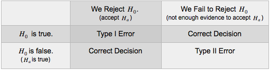
What Can Go Wrong: Two Types of Errors
Statistical investigations involve making decisions in the face of uncertainty, so there is always some chance of making a wrong decision. In hypothesis testing, two types of wrong decisions can occur.
If the null hypothesis is true, but we reject it, the error is a type I error.
If the null hypothesis is false, but we fail to reject it, the error is a type II error.
The following table summarizes type I and II errors.
Comment
Type I and type II errors are not caused by mistakes. These errors are the result of random chance. The data provide evidence for a conclusion that is false. It’s no one’s fault!
Example
Data Use on Smart Phones

In a previous example, we looked at a hypothesis test about data usage on smart phones. The researcher investigated the claim that the mean data usage for all teens is greater than 62 MBs. The sample mean was 75 MBs. The P-value was approximately 0.023. In this situation, the P-value is the probability that we will get a sample mean of 75 MBs or higher if the true mean is 62 MBs.
Notice that the result (75 MBs) isn’t impossible, only very unusual. The result is rare enough that we question whether the null hypothesis is true. This is why we reject the null hypothesis. But it is possible that the null hypothesis hypothesis is true and the researcher happened to get a very unusual sample mean. In this case, the result is just due to chance, and the data have led to a type I error: rejecting the null hypothesis when it is actually true.
Example
White Male Support for Obama in 2012
In a previous example, we conducted a hypothesis test using poll results to determine if white male support for Obama in 2012 will be less than 40%. Our poll of white males showed 35% planning to vote for Obama in 2012. Based on the sampling distribution, we estimated the P-value as 0.078. In this situation, the P-value is the probability that we will get a sample proportion of 0.35 or less if 0.40 of the population of white males support Obama.
At the 5% level, the poll did not give strong enough evidence for us to conclude that less than 40% of white males will vote for Obama in 2012.
Which type of error is possible in this situation? If, in fact, it is true that less than 40% of this population support Obama, then the data led to a type II error: failing to reject a null hypothesis that is false. In other words, we failed to accept an alternative hypothesis that is true.
We definitely did not make a type I error here because a type I error requires that we reject the null hypothesis.
Learn By Doing
Learn By Doing
What Is the Probability That We Will Make a Type I Error?
If the significance level is 5% (α = 0.05), then 5% of the time we will reject the null hypothesis (when it is true!). Of course we will not know if the null is true. But if it is, the natural variability that we expect in random samples will produce rare results 5% of the time. This makes sense because we assume the null hypothesis is true when we create the sampling distribution. We look at the variability in random samples selected from the population described by the null hypothesis.
Similarly, if the significance level is 1%, then 1% of the time sample results will be rare enough for us to reject the null hypothesis hypothesis. So if the null hypothesis is actually true, then by chance alone, 1% of the time we will reject a true null hypothesis. The probability of a type I error is therefore 1%.
In general, the probability of a type I error is α.
What Is the Probability That We Will Make a Type II Error?
The probability of a type I error, if the null hypothesis is true, is equal to the significance level. The probability of a type II error is much more complicated to calculate. We can reduce the risk of a type I error by using a lower significance level. The best way to reduce the risk of a type II error is by increasing the sample size. In theory, we could also increase the significance level, but doing so would increase the likelihood of a type I error at the same time. We discuss these ideas further in a later module.
Learn By Doing
A Fair Coin
In the long run, a fair coin lands heads up half of the time. (For this reason, a weighted coin is not fair.) We conducted a simulation in which each sample consists of 40 flips of a fair coin. Here is a simulated sampling distribution for the proportion of heads in 2,000 samples. Results ranged from 0.25 to 0.75.
 https://assessments.lumenlearning.co...sessments/3910
Comment
In general, if the null hypothesis is true, the significance level gives the probability of making a type I error. If we conduct a large number of hypothesis tests using the same null hypothesis, then, a type I error will occur in a predictable percentage (α) of the hypothesis tests. This is a problem! If we run one hypothesis test and the data is significant at the 5% level, we have reasonably good evidence that the alternative hypothesis is true. If we run 20 hypothesis tests and the data in one of the tests is significant at the 5% level, it doesn’t tell us anything! We expect 5% of the tests (1 in 20) to show significant results just due to chance.
Example
Cell Phones and Brain Cancer

The following is an excerpt from a 1999 New York Times article titled “Cell phones: questions but no answers,” as referenced by David S. Moore in Basic Practice of Statistics (4th ed., New York: W. H. Freeman, 2007):
- A hospital study that compared brain cancer patients and a similar group without brain cancer found no statistically significant association between cell phone use and a group of brain cancers known as gliomas. But when 20 types of glioma were considered separately, an association was found between cell phone use and one rare form. Puzzlingly, however, this risk appeared to decrease rather than increase with greater mobile phone use.
This is an example of a probable type I error. Suppose we conducted 20 hypotheses tests with the null hypothesis “Cell phone use is not associated with cancer” at the 5% level. We expect 1 in 20 (5%) to give significant results by chance alone when there is no association between cell phone use and cancer. So the conclusion that this one type of cancer is related to cell phone use is probably just a result of random chance and not an indication of an association.
Click here to see a fun cartoon that illustrates this same idea.
Learn By Doing
How Many People Are Telepathic?
Telepathy is the ability to read minds. Researchers used Zener cards in the early 1900s for experimental research into telepathy.
In a telepathy experiment, the “sender” looks at 1 of 5 Zener cards while the “receiver” guesses the symbol. This is repeated 40 times, and the proportion of correct responses is recorded. Because there are 5 cards, we expect random guesses to be right 20% of the time (1 out of 5) in the long run. So in 40 tries, 8 correct guesses, a proportion of 0.20, is common. But of course there will be variability even when someone is just guessing. Thirteen or more correct in 40 tries, a proportion of 0.325, is statistically significant at the 5% level. When people perform this well on the telepathy test, we conclude their performance is not due to chance and take it as an indication of the ability to read minds.
In the next section, “Hypothesis Test for a Population Proportion,” we learn the details of hypothesis testing for claims about a population proportion. Before we get into the details, we want to step back and think more generally about hypothesis testing. We close our introduction to hypothesis testing with a helpful analogy.
A Courtroom Analogy for Hypothesis Tests
When a defendant stands trial for a crime, he or she is innocent until proven guilty. It is the job of the prosecution to present evidence showing that the defendant is guilty beyond a reasonable doubt. It is the job of the defense to challenge this evidence to establish a reasonable doubt. The jury weighs the evidence and makes a decision.
When a jury makes a decision, it has only two possible verdicts:
- Guilty: The jury concludes that there is enough evidence to convict the defendant. The evidence is so strong that there is not a reasonable doubt that the defendant is guilty.
- Not Guilty: The jury concludes that there is not enough evidence to conclude beyond a reasonable doubt that the person is guilty. Notice that they do not conclude that the person is innocent. This verdict says only that there is not enough evidence to return a guilty verdict.
How is this example like a hypothesis test?
The null hypothesis is “The person is innocent.” The alternative hypothesis is “The person is guilty.” The evidence is the data. In a courtroom, the person is assumed innocent until proven guilty. In a hypothesis test, we assume the null hypothesis is true until the data proves otherwise.
The two possible verdicts are similar to the two conclusions that are possible in a hypothesis test.
Reject the null hypothesis: When we reject a null hypothesis, we accept the alternative hypothesis. This is like a guilty verdict. The evidence is strong enough for the jury to reject the assumption of innocence. In a hypothesis test, the data is strong enough for us to reject the assumption that the null hypothesis is true.
Fail to reject the null hypothesis: When we fail to reject the null hypothesis, we are delivering a “not guilty” verdict. The jury concludes that the evidence is not strong enough to reject the assumption of innocence, so the evidence is too weak to support a guilty verdict. We conclude the data is not strong enough to reject the null hypothesis, so the data is too weak to accept the alternative hypothesis.
How does the courtroom analogy relate to type I and type II errors?
Type I error: The jury convicts an innocent person. By analogy, we reject a true null hypothesis and accept a false alternative hypothesis.
Type II error: The jury says a person is not guilty when he or she really is. By analogy, we fail to reject a null hypothesis that is false. In other words, we do not accept an alternative hypothesis when it is really true.
Let’s Summarize
In this section, we introduced the four-step process of hypothesis testing:
Step 1: Determine the hypotheses.
- The hypotheses are claims about the population(s).
- The null hypothesis is a hypothesis that the parameter equals a specific value.
- The alternative hypothesis is the competing claim that the parameter is less than, greater than, or not equal to the parameter value in the null. The claim that drives the statistical investigation is usually found in the alternative hypothesis.
Step 2: Collect the data.
Because the hypothesis test is based on probability, random selection or assignment is essential in data production.
Step 3: Assess the evidence.
- Use the data to find a P-value.
- The P-value is a probability statement about how unlikely the data is if the null hypothesis is true.
- More specifically, the P-value gives the probability of sample results at least as extreme as the data if the null hypothesis is true.
Step 4: Give the conclusion.
- A small P-value says the data is unlikely to occur if the null hypothesis is true. We therefore conclude that the null hypothesis is probably not true and that the alternative hypothesis is true instead.
- We often choose a significance level as a benchmark for judging if the P-value is small enough. If the P-value is less than or equal to the significance level, we reject the null hypothesis and accept the alternative hypothesis instead.
- If the P-value is greater than the significance level, we say we “fail to reject” the null hypothesis. We never say that we “accept” the null hypothesis. We just say that we don’t have enough evidence to reject it. This is equivalent to saying we don’t have enough evidence to support the alternative hypothesis.
- Our conclusion will respond to the research question, so we often state the conclusion in terms of the alternative hypothesis.
Inference is based on probability, so there is always uncertainty. Although we may have strong evidence against it, the null hypothesis may still be true. If this is the case, we have a type I error. Similarly, even if we fail to reject the null hypothesis, it does not mean the alternative hypothesis is false. In this case, we have a type II error. These errors are not the result of a mistake in conducting the hypothesis test. They occur because of random chance.
- Concepts in Statistics. Provided by: Open Learning Initiative. Located at: http://oli.cmu.edu. License: CC BY: Attribution