3.7: Reading- Creating and Interpreting Graphs

Last updated
Save as PDF

Page ID: 249238

\( \newcommand{\vecs}[1]{\overset { \scriptstyle \rightharpoonup} {\mathbf{#1}} } \)

\( \newcommand{\vecd}[1]{\overset{-\!-\!\rightharpoonup}{\vphantom{a}\smash {#1}}} \)

\( \newcommand{\id}{\mathrm{id}}\) \( \newcommand{\Span}{\mathrm{span}}\)

( \newcommand{\kernel}{\mathrm{null}\,}\) \( \newcommand{\range}{\mathrm{range}\,}\)

\( \newcommand{\RealPart}{\mathrm{Re}}\) \( \newcommand{\ImaginaryPart}{\mathrm{Im}}\)

\( \newcommand{\Argument}{\mathrm{Arg}}\) \( \newcommand{\norm}[1]{\| #1 \|}\)

\( \newcommand{\inner}[2]{\langle #1, #2 \rangle}\)

\( \newcommand{\Span}{\mathrm{span}}\)

\( \newcommand{\id}{\mathrm{id}}\)

\( \newcommand{\Span}{\mathrm{span}}\)

\( \newcommand{\kernel}{\mathrm{null}\,}\)

\( \newcommand{\range}{\mathrm{range}\,}\)

\( \newcommand{\RealPart}{\mathrm{Re}}\)

\( \newcommand{\ImaginaryPart}{\mathrm{Im}}\)

\( \newcommand{\Argument}{\mathrm{Arg}}\)

\( \newcommand{\norm}[1]{\| #1 \|}\)

\( \newcommand{\inner}[2]{\langle #1, #2 \rangle}\)

\( \newcommand{\Span}{\mathrm{span}}\) \( \newcommand{\AA}{\unicode[.8,0]{x212B}}\)

\( \newcommand{\vectorA}[1]{\vec{#1}} % arrow\)

\( \newcommand{\vectorAt}[1]{\vec{\text{#1}}} % arrow\)

\( \newcommand{\vectorB}[1]{\overset { \scriptstyle \rightharpoonup} {\mathbf{#1}} } \)

\( \newcommand{\vectorC}[1]{\textbf{#1}} \)

\( \newcommand{\vectorD}[1]{\overrightarrow{#1}} \)

\( \newcommand{\vectorDt}[1]{\overrightarrow{\text{#1}}} \)

\( \newcommand{\vectE}[1]{\overset{-\!-\!\rightharpoonup}{\vphantom{a}\smash{\mathbf {#1}}}} \)

\( \newcommand{\vecs}[1]{\overset { \scriptstyle \rightharpoonup} {\mathbf{#1}} } \)

\( \newcommand{\vecd}[1]{\overset{-\!-\!\rightharpoonup}{\vphantom{a}\smash {#1}}} \)

\(\newcommand{\avec}{\mathbf a}\) \(\newcommand{\bvec}{\mathbf b}\) \(\newcommand{\cvec}{\mathbf c}\) \(\newcommand{\dvec}{\mathbf d}\) \(\newcommand{\dtil}{\widetilde{\mathbf d}}\) \(\newcommand{\evec}{\mathbf e}\) \(\newcommand{\fvec}{\mathbf f}\) \(\newcommand{\nvec}{\mathbf n}\) \(\newcommand{\pvec}{\mathbf p}\) \(\newcommand{\qvec}{\mathbf q}\) \(\newcommand{\svec}{\mathbf s}\) \(\newcommand{\tvec}{\mathbf t}\) \(\newcommand{\uvec}{\mathbf u}\) \(\newcommand{\vvec}{\mathbf v}\) \(\newcommand{\wvec}{\mathbf w}\) \(\newcommand{\xvec}{\mathbf x}\) \(\newcommand{\yvec}{\mathbf y}\) \(\newcommand{\zvec}{\mathbf z}\) \(\newcommand{\rvec}{\mathbf r}\) \(\newcommand{\mvec}{\mathbf m}\) \(\newcommand{\zerovec}{\mathbf 0}\) \(\newcommand{\onevec}{\mathbf 1}\) \(\newcommand{\real}{\mathbb R}\) \(\newcommand{\twovec}[2]{\left[\begin{array}{r}#1 \\ #2 \end{array}\right]}\) \(\newcommand{\ctwovec}[2]{\left[\begin{array}{c}#1 \\ #2 \end{array}\right]}\) \(\newcommand{\threevec}[3]{\left[\begin{array}{r}#1 \\ #2 \\ #3 \end{array}\right]}\) \(\newcommand{\cthreevec}[3]{\left[\begin{array}{c}#1 \\ #2 \\ #3 \end{array}\right]}\) \(\newcommand{\fourvec}[4]{\left[\begin{array}{r}#1 \\ #2 \\ #3 \\ #4 \end{array}\right]}\) \(\newcommand{\cfourvec}[4]{\left[\begin{array}{c}#1 \\ #2 \\ #3 \\ #4 \end{array}\right]}\) \(\newcommand{\fivevec}[5]{\left[\begin{array}{r}#1 \\ #2 \\ #3 \\ #4 \\ #5 \\ \end{array}\right]}\) \(\newcommand{\cfivevec}[5]{\left[\begin{array}{c}#1 \\ #2 \\ #3 \\ #4 \\ #5 \\ \end{array}\right]}\) \(\newcommand{\mattwo}[4]{\left[\begin{array}{rr}#1 \amp #2 \\ #3 \amp #4 \\ \end{array}\right]}\) \(\newcommand{\laspan}[1]{\text{Span}\{#1\}}\) \(\newcommand{\bcal}{\cal B}\) \(\newcommand{\ccal}{\cal C}\) \(\newcommand{\scal}{\cal S}\) \(\newcommand{\wcal}{\cal W}\) \(\newcommand{\ecal}{\cal E}\) \(\newcommand{\coords}[2]{\left\{#1\right\}_{#2}}\) \(\newcommand{\gray}[1]{\color{gray}{#1}}\) \(\newcommand{\lgray}[1]{\color{lightgray}{#1}}\) \(\newcommand{\rank}{\operatorname{rank}}\) \(\newcommand{\row}{\text{Row}}\) \(\newcommand{\col}{\text{Col}}\) \(\renewcommand{\row}{\text{Row}}\) \(\newcommand{\nul}{\text{Nul}}\) \(\newcommand{\var}{\text{Var}}\) \(\newcommand{\corr}{\text{corr}}\) \(\newcommand{\len}[1]{\left|#1\right|}\) \(\newcommand{\bbar}{\overline{\bvec}}\) \(\newcommand{\bhat}{\widehat{\bvec}}\) \(\newcommand{\bperp}{\bvec^\perp}\) \(\newcommand{\xhat}{\widehat{\xvec}}\) \(\newcommand{\vhat}{\widehat{\vvec}}\) \(\newcommand{\uhat}{\widehat{\uvec}}\) \(\newcommand{\what}{\widehat{\wvec}}\) \(\newcommand{\Sighat}{\widehat{\Sigma}}\) \(\newcommand{\lt}{<}\) \(\newcommand{\gt}{>}\) \(\newcommand{\amp}{&}\) \(\definecolor{fillinmathshade}{gray}{0.9}\)

It’s important to know the terminology of graphs in order to understand and manipulate them. Let’s begin with a visual representation of the terms (shown in Figure 1), and then we can discuss each one in greater detail.

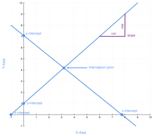
A standard graph with an x- and y-axis. There is a positive slope line and a negative slope line. Where the lines cross the x-axis is a x-intercept. Where the lines cross the y-axis is a y-intercept. Where the two lines cross is the intercept. Slope is defined as rise over run, or the slant of the line.

Figure 1. Graph Terminology

Throughout this course we will refer to the horizontal line on the graph as the x-axis. We will refer to the vertical line on the graph as the y-axis. This is the standard convention for graphs.

An intercept is where a line on a graph crosses (“intercepts”) the x-axis or the y-axis. You can see the x-intercepts and y-intercepts on the graph above. The point where two lines on a graph cross is called the interception point.

The other important term to know is slope. The slope tells us how steep a line on a graph is. Technically, slope is the change in the vertical axis divided by the change in the horizontal axis. The formula for calculating the slope is often referred to as the “rise over the run”—again, the change in the distance on the y-axis (rise) divided by the change in the x-axis (run).

Now that you know the “parts” of a graph, let’s turn to the equation for a line:

“> y = b + mx

Let’s use the same equation we used earlier, in the section on solving algebraic equations:

y = 9 + 3x

“>In this equation for a line, the b term is 9 and the m term is 3. The table below shows the values of x and y for this equation. To construct the table, just plug in a series of different values for x, and then calculate the resulting values for y.

Values for the Slope Intercept Equation
x	y
0	9
1	12
2	15
3	18
4	21
5	24
6	27

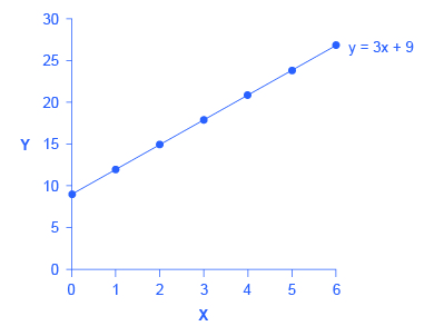
Next we can place each of these points on a graph. We can start with 0 on the x-axis and plot a point at 9 on the y-axis. We can do the same with the other pairs of values and draw a line through all the points, as on the graph in Figure 2, below.

The line graph shows the following approximate points: (0, 9); (1, 12); (2, 15); (3, 18); (4, 21); (5, 24); (6, 27).

Figure 2. Slope and Algebra of a Straight Line

This example illustrates how the b and m terms in an equation for a straight line determine the shape of the line. The b term is called the y-intercept. The reason is that if x = 0, the b term will reveal where the line intercepts, or crosses, the y-axis. In this example, the line hits the vertical axis at 9. The m term in the equation for the line is the slope. Remember that slope is defined as rise over run; the slope of a line from one point to another is the change in the vertical axis divided by the change in the horizontal axis. In this example, each time the x term increases by 1 (the run), the y term rises by 3. Thus, the slope of this line is 3. Specifying a y-intercept and a slope—that is, specifying b and m in the equation for a line—will identify a specific line. Although it is rare for real-world data points to arrange themselves as a perfectly straight line, it often turns out that a straight line can offer a reasonable approximation of actual data.

Revision and adaptation. Provided by: Lumen Learning. License: CC BY: Attribution

Principles of Microeconomics Appendix. Authored by: OpenStax. Provided by: Rice University. Located at: http://cnx.org/contents/6i8iXmBj@10.170:Nihva8h5@10/The-Use-of-Mathematics-in-Prin. License: CC BY: Attribution. License Terms: Download for free at http://cnx.org/content/col11627/latest

Search

Text Color

Text Size

Margin Size

Font Type