2603 Rate Law and the Initial Rate Method

1.0 INTRODUCTION

1.1 Objectives

After completing this experiment, the student will be able to:

• determine the rate law of a chemical reaction using the initial rate method.
• determine the energy of activation (Ea) of the reaction by finding the value of the rate constant, k, at different temperatures.

1.2 Background

1.2.1 Finding the Rate Law using the Initial Rate Method

The rate law of a chemical reaction is a mathematical equation that describes how the reaction rate depends upon the concentration of each reactant. Two methods are commonly used in the experimental determination of the rate law: the initial rate method and the graphical method. In this experiment, we shall use the initial rate method to determine the rate law of a reaction. It will be helpful to review this concept in the lecture.

The reaction to be studied in this experiment is represented by the following balanced ionic equation:

6 I-(aq) + BrO3-(aq) + 6 H+(aq) 🡪 3 I2(aq) + Br-(aq) + 3 H2O(l) (Equation 1)

The rate law for this reaction is of the form:

rate = k [I-]m[BrO3-]n[H+]p (Equation 2)

where the value of the rate constant, k, is dependent upon the temperature at which the

reaction is run. The values of the reaction orders, m, n, and p are usually, though not always, small integers. The values of m, n, p and k must be determined experimentally to specify the rate law for this reaction completely.

The initial rate method allows the values of the reaction orders to be found by running the reaction multiple times under controlled conditions and measuring the rate of the reaction in each case. All variables are held constant from one run to the next, except for the concentration of one reactant. The order of that reactant concentration in the rate law can be determined by observing how the reaction rate varies as the concentration of that one reactant is varied. This method is repeated for each reactant until all the orders are determined. At that point, the rate law can be used to find the value of k for each trial. If the temperatures are the same for each trial, then the values of k should be the same too.

The rate of the reaction can be expressed in terms of the rate of decrease of the concentration of BrO3-.

rate of reaction=-∆[BrO3-]/∆t (Equation 3)

Note that this is the average rate of the reaction over the time interval Δt since the concentration of BrO3- and therefore the rate of the reaction is continuously decreasing during Δt. In this experiment, we can assume that Δ[BrO3-] is negligible compared to [BrO3-] thus allowing us to approximate our measured average rate as being equal to the initial, instantaneous rate.

In addition, the rate of the reaction will be measured indirectly by running a second reaction, known as a ‘clock’ reaction, simultaneously along with the reaction of interest. The ‘clock’ reaction must be inherently fast relative to the reaction of interest, and it must consume at least one of the products (I2) of the reaction of interest. In this case, the parallel reactions are the following:

6 I-(aq) + BrO3-(aq) + 6 H+(aq) 🡪 3 I2(aq) + Br-(aq) + 3 H2O(l) slow

(‘clock’ reaction) 3 I2(aq) + 6 S2O32-(aq) 🡪 6 I-(aq) + 3 S4O62-(aq) fast

Overall reaction:

BrO3-(aq) + 6 S2O32-(aq) + 6 H+(aq) 🡪 Br-(aq) + 3 H2O(l) + 3 S4O62-(aq) (Equation 4)

Note that since the ‘clock’ reaction is relatively fast, the I2(aq) will be consumed by the clock reaction as quickly as it can be produced by the reaction of interest thus holding the I2 concentration at a very low value close to zero. Only after the S2O32- has been entirely consumed will the concentration of I2 start to increase. After the S2O32- has been consumed, the concentration of I2 will increase rapidly allowing the I2 to react with a starch indicator resulting in the solution to acquire a deep blue color.

In this experiment, you will measure the time required for the solution to turn blue.

This is essentially the amount of time required for all the S2O32- to be reacted.

A stoichiometric calculation can be used to determine the number of moles of BrO3- reacted at the point in time when all the S2O32- has been consumed. By dividing the number of moles of BrO3- reacted by the total volume of the reaction mixture we can obtain the change in the BrO3- concentration. We can obtain the reaction rate by dividing this change in concentration by the amount of time required for the blue color to appear (Δt).

1. Measure the time required for the solution to turn blue. (all S2O32- reacted)
2. Calculate moles BrO3- reacted
3. Divide moles BrO3- by total volume of reaction mixture = [BrO3-]
4. Reaction rate = [BrO3-] divided by a. = [BrO3-]/(Δt)

1.2.2 Determining the Activation Energy of the Reaction

The value of the rate constant, k, measured previously is dependent upon the

temperature at which the reaction occurs according to the Arrhenius Equation:

_k=Ae-Ea/RT (Equation 5)

where A is the frequency factor and is related to the number of properly aligned collisions

that occur per second between reactant molecules; Ea is the activation energy of the

reaction and is the minimum energy that must be present in a collision for a reaction to

occur; and R is the universal gas constant with a value of 8.3145 x 10-3 kJ·mol–1.

Taking the natural logarithm of both sides of Equation 5 gives:

ln ln k=-E_a/R (1/T)+ln ln A (Equation 6)

Note that this equation is that of a straight line of the form, y=mx+b, where:

y=ln k , x=1/T , m=-E_a/R , and b=ln ln A .

Thus, if the rate constant, k, is measured at several temperatures and ln k is plotted as a

function of 1/T, the slope of the resulting line will allow the value of Ea for the reaction to be determined.

2.0 SAFETY PRECAUTIONS AND WASTE DISPOSAL

3.0 CHEMICALS AND SolutionS

3.0 CHEMICALS AND SolutionS

Chemical	Concentration	Approximate Amount	Notes
Laboratory water	Pure	150 mL	Be sure to use laboratory water
KI(aq)	0.010 M	100 mL
Na2S2O3(aq)	0.0010 M	100 mL
KBrO3(aq)	0.040 M	100 mL
HCl(aq)	0.10 M	100 mL
Ice	Pure		For preparing ice/water bath
Starch solution	0.5 – 1 %	3-4 drops for each reaction mixture	For use as indicator

4.0 GLASSWARE AND APPARATUS

Squirt bottle	10 mL graduated cylinder
250 mL beakers (4) (or any size ≥ 150 mL)	Large test tubes (2)
250 mL Erlenmeyer flask	600 or 1000 mL beaker (for the hot water bath)
125 mL Erlenmeyer flask	Thermometer
Medium test tubes (4)	Hot plate

5.0 PROCEDURE

5.1 Preparation of Glassware

• Because soap residue and other chemicals can interfere with the reaction we are observing, it is critical that all glassware used in this experiment be rinsed several times using laboratory water (and not soap!) prior to performing the experiment. Use a squirt bottle to minimize waste; never rinse glassware directly under the laboratory water tap. In general, there is no need to dry glassware after rinsing because most solutions that we use are aqueous. But shake them gently several times to remove almost all the water.
• Prior to use, make sure to rinse the graduated cylinder with about 2-3 mL of the reagent, pouring this rinse into the sink.

5.2 Determining the Rate Law Using the Initial Rate Method

As shown in the table below, four (4) reaction mixtures will be prepared. The table summarizes the volume of each reagent that should be used in each reaction mixture.

Reaction Mixture	Flask I (250 mL)			Flask II (125 mL)
	0.010 M KI	0.0010 M Na2S2O3	Laboratory H2O	0.040 M KBrO3	0.10 M HCl	1% Starch
1	10.0 mL	10.0 mL	10.0 mL	10.0 mL	10.0 mL	3-4 drops
2	20.0 mL	10.0 mL	---	10.0 mL	10.0 mL	3-4 drops
3	10.0 mL	10.0 mL	---	20.0 mL	10.0 mL	3-4 drops
4	10.0 mL	10.0 mL	---	10.0 mL	20.0 mL	drops

1. Using the four 250-mL beakers (or any size ≥ 150 mL available), obtain about 100 mL of each of the four reagents needed to prepare the mixtures listed in the table (except laboratory water). Rinse each beaker with about 5 mL of the particular reagent solution you will store in it first, pouring this rinse into the sink, then fill the beaker with the 100 mL you will need. Label each beaker appropriately. You are now ready to prepare Reaction Mixture 1.
2. Using a clean 10-mL graduated cylinder, measure 10.0 mL of laboratory water (from your squirt bottle) and transfer it into the 250-mL Erlenmeyer flask (labeled Flask I).
3. Into the 250-mL Erlenmeyer flask containing the 10.0 mL of laboratory water (Flask I), separately measure and add 10.0 mL of the 0.010 M KI and 10.0 mL of the 0.0010 M Na2S2O3.
4. Into the 125-mL Erlenmeyer flask (labeled Flask II), in a similar manner, combine 10.0 mL of the 0.040 M KBrO3 reagent solution, 10.0 mL of the 0.10 M HCl solution, and 3 to 4 drops of starch indicator. Shake the starch solution thoroughly before use.
5. The next step requires two experimenters: one to operate the stopwatch or timer and another to mix and swirl the contents of the two flasks. Be certain that the person using the stopwatch or timer knows how to operate it by testing it once or twice before proceeding.
6. Pour the contents of Flask II into Flask I rapidly and then swirl the solution to mix thoroughly. Start your stopwatch or timer the moment the two solutions are combined. Set the flask containing the reaction mixture down on a sheet of white paper and watch carefully for the blue color of the starch-iodine complex to appear. It should take about one to three minutes. Stop the timer the instant that the blue color appears. Record the elapsed time on your data recording sheet.
7. Using your thermometer, measure the temperature of the reaction mixture immediately following the reaction to the nearest tenth of a degree and record this value on your data recording sheet.
8. Dispose of the contents of the flask in the sink. Rinse both Erlenmeyer flasks and your thermometer as described in the preparation of glassware section (Part 5.1).
9. Repeat steps 2 to 7, performing a second trial for Reaction Mixture 1. If the time you measure for this second trial differs by more than 10% from that of your first trial, repeat the procedure. If after three trials you still unable to obtain two trials with reaction times that differ by less than 10%, see your instructor.
10. Now repeat this procedure for the other three reaction mixtures listed in the table above. You need to perform only one trial for each of these mixtures. Compare the times you obtain for each of these mixtures with those obtained by other teams. Repeat any trials where the reaction time differs significantly from those obtained by other teams. Record these data on your data recording sheet. Do not forget to measure the temperature immediately following each trial.
11. Dispose of the contents of the flasks in the sink. Rinse the flasks, and thermometer before returning into your locker or to the stockroom.

5.3 Determining the Activation Energy (Ea) of the Reaction (Optional)

1. Prepare the solutions given for Reaction Mixture 1 in the table but instead of a 250 mL Erlenmeyer flask, use large test tubes (labeled TT 1 and TT 2).

2. Prepare a water bath at room temperature using tap water and a large (600 mL or 1000 mL) beaker. Use utility clamps to secure the large test tubes, and a thermometer into the water bath. Make sure that the solution levels are at or below the water bath level. Let them sit for about five minutes to equilibrate to the bath temperature. After equilibration, record the water bath temperature on your data recording sheet. This will be the reaction temperature.

3. Remove TT 1 from the clamp and quickly transfer the solution into TT 2. Swirl the reaction mixture to mix thoroughly. Start your timer the moment you combine the two solutions. Keep the flask containing the mixed solution in the water bath and observe carefully for the blue color to appear. Stop the timer the instant that this faint blue color first appears. Record the elapsed time and the final temperature of this mixture on your data recording sheet.

4. Dispose of the contents of the flask in the sink. Rinse the 125 mL Erlenmeyer flask and your thermometer as described in the preparation of glassware section (Part 5.1). The test tube does not need to be cleaned since it will always contain the same solution mixture.

5. Perform two more trials at elevated temperatures using a hot-water bath in place of the room temperature water bath. Each trial should be performed using the quantities given for Reaction Mixture 1 in the table. Heat both test tube and 125 mL Erlenmeyer flask in a hot-water bath (on a hot plate) until the temperature in the water bath reaches approximately 30°C (±5°C) in the first elevated-temperature trial, and about 40°C (±5°C) in the second elevated-temperature trial. When the appropriate temperature has been reached, remove the flasks, mix the contents, and record the elapsed time for the blue color to appear. Record the final temperature of the reaction mixture as before. (If time permits, you can perform a low temperature run by preparing an ice/water bath that is between 10oC and 15oC.)

6. Dispose of the contents of the test tubes in the sink. Rinse the test tubes, and thermometer before returning into your locker or to the stockroom.

6.0 DATA RECORDING SHEET

Last Name

First Name

Partner Name(s)

Date

6.1 Determining the Rate Law Using the Initial Rate Method

Reaction Mixture 1 (to confirm constancy between trials)

Trial	Elapsed Time, Δt (s)	Temperature (oC)	Notes/Observations
1
2
3 (if needed)
Average

Data for Reaction Mixtures 1 through 4

Reaction Mixture	Elapsed time, Δt (s)	Temperature (oC)	Notes/Observations
1 (avg from above)
2
3
4

6.2 Determining the Activation Energy, Ea, of the Reaction

Data for the Effect of Temperature on the Reaction Rate (Reaction Mixture 1)

	Low Temp	Room Temp	About 30oC	About 40oC
Temp of Reaction Mixture (oC)
Temp of Reaction Mixture (K)
Elapsed time, Δt (s)

7.0 CALCULATIONS

7.1 Initial Concentrations of the Reactants After Mixing

Use the dilution equation, M1V1 = M2V2 to calculate the initial concentration of each reagent after preparing the reaction mixture.

Reaction Mixture	[I-]o (M)	[S2O32-]o (M)	[BrO3-]o (M)	[H+]o (M)
1
2
3
4

Show your calculations below for each reagent in one of the reaction mixtures.

7.2 Relative Rates of Reaction

1. Based on the stoichiometry of the reaction in Equation 4, fill in the values of a and b in the relative rate expression:

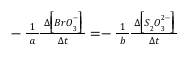
Relative rate expression: ___________________________________

2. Use your concentration and time (elapsed time) data from the previous section (Part 7.1) to calculate the rate that S2O32– is consumed in each of your four mixtures. Then, use the relative rate expression above to determine the corresponding initial rate of reaction in terms of the change in concentration of BrO3– reacted.

Relative rates of reaction

Reaction Mixture
1
2
3
4

Show your calculations below for one of the reaction mixtures.

7.3 Order of the Reaction with Respect to Each Reactant and the Rate Law

1. Copy (from Parts 7.1 and 7.2) the appropriate values of the initial reactant concentrations and reaction rates in the table below.

Reaction Mixture	[I-]o (M)	[BrO3-]o (M)	[H+]o (M)	Rate (M/s)
1
2
3
4

2. Using the initial rate method and the relevant data in the table above, determine the order of the reaction with respect to each reactant, and then write the experimentally determined rate law for the reaction (Equation 2). Show all your calculations below, noting the reaction mixtures used for your data.

Reaction order with respect to I-:

Reaction order with respect to BrO3-:

Reaction order with respect to H+:

Rate law: ______________________________________

7.4 Value of the Rate Constant, k

Using your experimentally determined rate law from Part 7.3, determine the value of the rate constant, k, for each reaction mixture and then, calculate its average. Observe proper significant figures and units.

Reaction Mixture	Value of k	Average value of k
1
2
3
4

Show your calculations below illustrating how you determined the value of k for one of the reaction mixtures.

7.5 Determining the Activation Energy, Ea, for the Reaction

1. Determine the value of the rate constant, k, for each temperature below and give the appropriate units.

	Low Temp	Room Temp	About 30oC	About 40oC
Rate constant, k
ln k (no units)
1/T (K-1)

Show your calculations for one of the reaction temperatures below:

2. Use Excel to create a graph of “ln k versus 1/T”. Your graph should have an appropriate title and labeled axes with an appropriate scale. Using the Excel trendline function, add a best-fit line to your plotted data and display the equation of this line and its R2 value on your graph. Submit this graph with your report.

Use this graph to determine the value of the activation energy, Ea, and the frequency factor, A, for this reaction (Be certain to include the proper units for each!). Show your calculations below.

8.0 POST-LAB QUESTIONS

1. The volume of each the reagents listed in the table (Part 5.2) are varied one at a time in turn except for the volume of sodium thiosulfate, which is the same in each trial. Why do we keep the volume of sodium thiosulfate the same in each trial?

2. Based on your calculations in Part 7.4, even though the concentrations of the reactants are changed in each reaction mixture, the experimentally determined values of the rate constant, k, should be fairly similar. Why is this?

3. Discuss the trend you observed from your graph in Part 7.5. Provide a physical explanation to explain this? What is occurring on the molecular level?