3.18: Application to the Rotation of Real Molecules

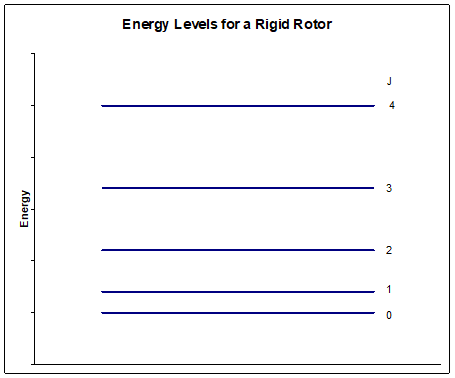
While the spherical harmonics are the wavefunctions that describe the rotational motion of a rigid rotator, the names of the quantum numbers are changed to reflect the type of angular momentum encountered in the problem. The quantum number \(l\) and \(m_{l}\) should be familiar as these are the ones used in the hydrogen atom problem to describe the orbital angular momentum. However, for rotational motion, these are replaced by \(\mathrm{J}\) and \(\mathrm{M}_{\mathrm{J}}\). The energy levels of the rigid rotator are therefore given by

\[E_{J}=J(J+1) \dfrac{\hbar^{2}}{2 \mu r^{2}}\nonumber\]

And since \(\mathrm{M}_{\mathrm{J}}\) does not appear in the energy level expression, each level has a \((2 \mathrm{~J}+1)\) degeneracy. The spacings between energy levels increases with increasing \(\mathrm{J}\) due to the \(\mathrm{J}(\mathrm{J}+1)\) dependence (which has a \(\mathrm{J}^{2}\) term.) This pattern is shown in the diagram below.

Figure \(\PageIndex{1}\)

For spectroscopic measurements, the rotational energy (given the symbol \(F_{J}\) ) is often expressed in spectroscopic units, such as \(\mathrm{cm}^{-1}\). Also, a spectroscopic constant, B, is used to describe the energy level stack.

\[F_{J}=\dfrac{E_{J}}{h c}=B J(J+1)\nonumber\]

where the spectroscopic constant \(B\) is given by

\[B=\dfrac{h}{8 \pi^{2} c \mu r^{2}}\nonumber\]

Thus, by knowing the value of \(\mu\), the reduced mass, and measuring the value of \(B\), the rotational constant, one can determine the value of \(\mathrm{r}\), the bond length. This is the utility of rotational spectroscopy - it gives us detailed information about molecular structure!

Centrifugal Distortion

As we know, since they vibrate, real molecules do not have rigid bonds. So it is no surprise to learn that the Rigid Rotor is really just a limiting ideal model, much like the ideal gas law describes limiting ideal behavior.

Real molecules, especially when rotating with very high angular momentum, will tend to stretch. In other words, the average bond length will increase with increasing \(J\). And given the inverse relationship between \(\mathrm{B}\) and bond length(\(r\)), it is not surprising that the effective \(B\) value is smaller at higher levels of \(\mathrm{J}\). In fact, this centrifugal distortion problem is well treated by introducing a "distortion constant" \(D\) such that

\[F_{J}=B J(J+1)-D[J(J+1)]^{2}\nonumber\]

Naturally, one would expect the distortion constant to be small in the case of a strong, inflexible bond, but larger if the bond is weaker. The approximation of Kraitzer suggests that the distortion constant is determined to a good approximation by

\[D \approx \dfrac{4 B^{3}}{\omega_{e}^{2}}\nonumber\]

For a well behaved molecule, he distortion constant \(\mathrm{D}\) is always smaller in magnitude than \(\mathrm{B}\). Some molecules require several distortional constants to yield a reasonable description of their rotational energy level stack. If additional constants are needed, they are introduced as coefficients in a power series of \(\mathrm{J}(\mathrm{J}+1)\).

\[\mathrm{F}_{\mathrm{J}}=\mathrm{BJ}(\mathrm{J}+1)-\mathrm{D}[\mathrm{J}(\mathrm{J}+1)]^{2}+\mathrm{H}[\mathrm{J}(\mathrm{J}+1)]^{3}+\ldots\nonumber\]

The power series is truncated at a point that yields a good fit to experimental observations for a given molecule.