13.6: F- Matrices

Definitions

An \(n \times m\) matrix is a two dimensional array of numbers with \(n\) rows and \(m\) columns. The integers \(n\) and \(m\) are called the dimensions of the matrix. If \(n = m\) then the matrix is square. The numbers in the matrix are known as matrix elements (or just elements) and are usually given subscripts to signify their position in the matrix e.g. an element \(a_{ij}\) would occupy the \(i^{th}\) row and \(j^{th}\) column of the matrix. For example:

\[M = \left(\begin{array}{ccc} 1 & 2 & 3 \\ 4 & 5 & 6 \\ 7 & 8 & 9 \end{array}\right) \label{8.1}\]

is a \(3 \times 3\) matrix with \(a_{11}=1\), \(a_{12}=2\), \(a_{13}=3\), \(a_{21}=4\) etc

In a square matrix, diagonal elements are those for which \(i\)=\(j\) (the numbers \(1\), \(5\), and \(9\) in the above example). Off-diagonal elements are those for which \(i \neq j\) (\(2\), \(3\), \(4\), \(6\), \(7\), and \(8\) in the above example). If all the off-diagonal elements are equal to zero then we have a diagonal matrix. We will see later that diagonal matrices are of considerable importance in group theory.

A unit matrix or identity matrix (usually given the symbol \(I\)) is a diagonal matrix in which all the diagonal elements are equal to \(1\). A unit matrix acting on another matrix has no effect – it is the same as the identity operation in group theory and is analogous to multiplying a number by \(1\) in everyday arithmetic.

The transpose \(A^T\) of a matrix \(A\) is the matrix that results from interchanging all the rows and columns. A symmetric matrix is the same as its transpose (\(A^T=A\) i.e. \(a_{ij} = a_{ji}\) for all values of \(i\) and \(j\)). The transpose of matrix \(M\) above (which is not symmetric) is

\[M^{T} = \left(\begin{array}{ccc} 1 & 4 & 7 \\ 2 & 5 & 8 \\ 3 & 6 & 9 \end{array}\right) \label{8.2}\]

The sum of the diagonal elements in a square matrix is called the trace (or character) of the matrix (for the above matrix, the trace is \(\chi = 1 + 5 + 9 = 15\)). The traces of matrices representing symmetry operations will turn out to be of great importance in group theory.

A vector is just a special case of a matrix in which one of the dimensions is equal to \(1\). An \(n \times 1\) matrix is a column vector; a \(1 \times m\) matrix is a row vector. The components of a vector are usually only labeled with one index. A unit vector has one element equal to \(1\) and the others equal to zero (it is the same as one row or column of an identity matrix). We can extend the idea further to say that a single number is a matrix (or vector) of dimension \(1 \times 1\).

Matrix Algebra

1. Two matrices with the same dimensions may be added or subtracted by adding or subtracting the elements occupying the same position in each matrix. e.g.

\[A = \begin{pmatrix} 1 & 0 & 2 \\ 2 & 2 &1 \\ 3 & 2 & 0 \end{pmatrix} \label{8.3}\]

\[B = \begin{pmatrix} 2 & 0 & -2 \\ 1 & 0 & 1 \\ 1 & -1 & 0 \end{pmatrix} \label{8.4}\]

\[A + B = \begin{pmatrix} 3 & 0 & 0 \\ 3 & 2 & 2 \\ 4 & 1 & 0 \end{pmatrix} \label{8.5}\]

\[A - B = \begin{pmatrix} -1 & 0 & 4 \\ 1 & 2 & 0 \\ 2 & 3 & 0 \end{pmatrix} \label{8.6}\]

2. A matrix may be multiplied by a constant by multiplying each element by the constant.

\[4B = \left(\begin{array}{ccc} 8 & 0 & -8 \\ 4 & 0 & 4 \\ 4 & -4 & 0 \end{array}\right) \label{8.7}\]

\[3A = \left(\begin{array}{ccc} 3 & 0 & 6 \\ 6 & 6 & 3 \\ 9 & 6 & 0 \end{array}\right) \label{8.8}\]

3. Two matrices may be multiplied together provided that the number of columns of the first matrix is the same as the number of rows of the second matrix i.e. an \(n \times m\) matrix may be multiplied by an \(m \times l\) matrix. The resulting matrix will have dimensions \(n \times l\). To find the element \(a_{ij}\) in the product matrix, we take the dot product of row \(i\) of the first matrix and column \(j\) of the second matrix (i.e. we multiply consecutive elements together from row \(i\) of the first matrix and column \(j\) of the second matrix and add them together i.e. \(c_{ij}\) = \(\Sigma_k\) \(a_{ik}\)\(b_{jk}\) e.g. in the \(3 \times 3\) matrices \(A\) and \(B\) used in the above examples, the first element in the product matrix \(C = AB\) is \(c_{11}\) = \(a_{11}\)\(b_{11}\) + \(a_{12}\)\(b_{21}\) + \(a_{13}\)\(b_{31}\)

\[AB = \begin{pmatrix} 1 & 0 & 2 \\ 2 & 2 & 1 \\ 3 & 2 & 0 \end{pmatrix} \begin{pmatrix} 2 & 0 & -2 \\ 1 & 0 & 1 \\ 1 & -1 & 0 \end{pmatrix} = \begin{pmatrix} 4 & -2 & -2 \\ 7 & -1 & -2 \\ 8 & 0 & -4 \end{pmatrix} \label{8.9}\]

An example of a matrix multiplying a vector is

\[A\textbf{v} = \begin{pmatrix} 1 & 0 & 2 \\ 2 & 2 & 1 \\ 3 & 2 & 0 \end{pmatrix} \begin{pmatrix} 1 \\ 2 \\ 3 \end{pmatrix} = \begin{pmatrix} 7 \\ 9 \\ 7 \end{pmatrix} \label{8.10}\]

Matrix multiplication is not generally commutative, a property that mirrors the behavior found earlier for symmetry operations within a point group.

Direct Products

The direct product of two matrices (given the symbol \(\otimes\)) is a special type of matrix product that generates a matrix of higher dimensionality if both matrices have dimension greater than one. The easiest way to demonstrate how to construct a direct product of two matrices \(A\) and \(B\) is by an example:

\[ \begin{align} A \otimes B &= \begin{pmatrix} a_{11} & a_{12} \\ a_{21} & a_{22} \end{pmatrix} \otimes \begin{pmatrix} b_{11} & b_{12} \\ b_{21} & b_{22} \end{pmatrix} \\[4pt] &= \begin{pmatrix} a_{11}B & a_{12}B \\ a_{21}B & a_{22}B \end{pmatrix} \\[4pt] &= \begin{pmatrix} a_{11}b_{11} & a_{11}b_{12} & a_{12}b_{11} & a_{12}b_{12} \\ a_{11}b_{21} & a_{11}b_{22} & a_{12}b_{21} & a_{12}b_{22} \\ a_{21}b_{11} & a_{21}b_{12} & a_{22}b_{11} & a_{22}b_{21} \\ a_{21}b_{21} & a_{21}b_{22} & a_{22}b_{21} & a_{22}b_{22} \end{pmatrix} \label{8.11} \end{align} \]

Though this may seem like a somewhat strange operation to carry out, direct products crop up a great deal in group theory.

Inverse Matrices and Determinants

If two square matrices \(A\) and \(B\) multiply together to give the identity matrix I (i.e. \(AB = I\)) then \(B\) is said to be the inverse of \(A\) (written \(A^{-1}\)). If \(B\) is the inverse of \(A\) then \(A\) is also the inverse of \(B\). Recall that one of the conditions imposed upon the symmetry operations in a group is that each operation must have an inverse. It follows by analogy that any matrices we use to represent symmetry elements must also have inverses. It turns out that a square matrix only has an inverse if its determinant is non-zero. For this reason (and others which will become apparent later on when we need to solve equations involving matrices) we need to learn a little about matrix determinants and their properties.

For every square matrix, there is a unique function of all the elements that yields a single number called the determinant. Initially it probably won’t be particularly obvious why this number should be useful, but matrix determinants are of great importance both in pure mathematics and in a number of areas of science. Historically, determinants were actually around before matrices. They arose originally as a property of a system of linear equations that ‘determined’ whether the system had a unique solution. As we shall see later, when such a system of equations is recast as a matrix equation this property carries over into the matrix determinant.

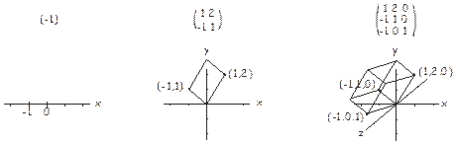
There are two different definitions of a determinant, one geometric and one algebraic. In the geometric interpretation, we consider the numbers across each row of an \(n \times n\) matrix as coordinates in \(n\)-dimensional space. In a one-dimensional matrix (i.e. a number), there is only one coordinate, and the determinant can be interpreted as the (signed) length of a vector from the origin to this point. For a \(2 \times 2\) matrix we have two coordinates in a plane, and the determinant is the (signed) area of the parallelogram that includes these two points and the origin. For a \(3 \times 3\) matrix the determinant is the (signed) volume of the parallelepiped that includes the three points (in three-dimensional space) defined by the matrix and the origin. This is illustrated below. The idea extends up to higher dimensions in a similar way. In some sense then, the determinant is therefore related to the size of a matrix.

The algebraic definition of the determinant of an \(nxn\) matrix is a sum over all the possible products (permutations) of n elements taken from different rows and columns. The number of terms in the sum is \(n!\), the number of possible permutations of \(n\) values (i.e. \(2\) for a \(2 \times 2\) matrix, \(6\) for a \(3 \times 3\) matrix etc). Each term in the sum is given a positive or a negative sign depending on whether the number of permutation inversions in the product is even or odd. A permutation inversion is just a pair of elements that are out of order when described by their indices. For example, for a set of four elements \(\begin{pmatrix} a_1, a_2, a_3, a_4 \end{pmatrix}\), the permutation \(a_1 a_2 a_3 a_4\) has all the elements in their correct order (i.e. in order of increasing index). However, the permutation \(a_2 a_4 a_1 a_3\) contains the permutation inversions \(a_2 a_1\), \(a_4 a_1\), \(a_4 a_3\).

For example, for a two-dimensional matrix

\[\begin{pmatrix} a_{11} & a_{12} \\ a_{21} & a_{22} \end{pmatrix} \label{8.12}\]

where the subscripts label the row and column positions of the elements, there are \(2\) possible products/permutations involving elements from different rows and column, \(a_{11}\)\(a_{22}\) and \(a_{12}\)\(a_{21}\). In the second term, there is a permutation inversion involving the column indices \(2\) and \(1\) (permutation inversions involving the row and column indices should be looked for separately) so this term takes a negative sign, and the determinant is \(a_{11}\)\(a_{22}\) - \(a_{12}\)\(a_{21}\).

For a \(3 \times 3\) matrix

\[\begin{pmatrix} a_{11} & a_{12} & a_{13} \\ a_{21} & a_{22} & a_{23} \\ a_{31} & a_{32} & a_{33} \end{pmatrix} \label{8.13}\]

the possible combinations of elements from different rows and columns, together with the sign from the number of permutations required to put their indices in numerical order are:

\[\begin{array}{rl}a_{11} a_{22} a_{33} & (0 \: \text{inversions}) \\ -a_{11} a_{23} a_{32} & (1 \: \text{inversion -} \: 3>2 \: \text{in the column indices}) \\ -a_{12} a_{21} a_{33} & (1 \: \text{inversion -} \: 2>1 \: \text{in the column indices}) \\ a_{12} a_{23} a_{31} & (2 \: \text{inversions -} \: 2>1 \: \text{and} \: 3>1 \: \text{in the column indices}) \\ a_{13} a_{21} a_{32} & (2 \: \text{inversions -} \: 3>1 \: \text{and} \: 3>2 \: \text{in the column indices}) \\ -a_{13} a_{22} a_{31} & (3 \: \text{inversions -} \: 3>2, 3>1, \: \text{and} \: 2>1 \: \text{in the column indices}) \end{array} \label{8.14}\]

and the determinant is simply the sum of these terms.

This may all seem a little complicated, but in practice there is a fairly systematic procedure for calculating determinants. The determinant of a matrix \(A\) is usually written det(\(A\)) or |\(a\)|.

For a \(2 \times 2\) matrix

\[A = \begin{pmatrix} a & b \\ c & d \end{pmatrix}; det(A) = |A| = \begin{vmatrix} a & b \\ c & d \end{vmatrix} = ad - bc \label{8.15}\]

For a \(3 \times 3\) matrix

\[B = \begin{pmatrix} a & b & c \\ d & e & f \\ g & h & i \end{pmatrix}; det(B) = a\begin{vmatrix} e & f \\ h & i \end{vmatrix} - b\begin{vmatrix} d & f \\ g & i \end{vmatrix} + c\begin{vmatrix} d & e \\ g & h \end{vmatrix} \label{8.16}\]

For a \(4x4\) matrix

\[C = \begin{pmatrix} a & b & c & d \\ e & f & g & h \\ i & j & k & l \\ m & n & o & p \end{pmatrix}; det(C) = a\begin{vmatrix} f & g & h \\ j & k & l \\ n & o & p \end{vmatrix} - b\begin{vmatrix} e & g & h \\ i & k & l \\ m & o & p \end{vmatrix} + c\begin{vmatrix} e & f & h \\ i & j & l \\ m & n & p \end{vmatrix} - d\begin{vmatrix} e & f & g \\ i & j & k \\ m & n & o \end{vmatrix} \label{8.17}\]

and so on in higher dimensions. Note that the submatrices in the \(3 \times 3\) example above are just the matrices formed from the original matrix \(B\) that don’t include any elements from the same row or column as the premultiplying factors from the first row.

Matrix determinants have a number of important properties:

1. The determinant of the identity matrix is \(1\).

\[e.g. \begin{vmatrix} 1 & 0 \\ 0 & 1 \end{vmatrix} = \begin{vmatrix} 1 & 0 & 0 \\ 0 & 1 & 0 \\ 0 & 0 & 1 \end{vmatrix} = 1 \label{8.18}\]

2. The determinant of a matrix is the same as the determinant of its transpose i.e. det(\(a\)) = det(\(A^{T}\))

\[e.g. \begin{vmatrix} a & b \\ c & d \end{vmatrix} = \begin{vmatrix} a & c \\ b & d \end{vmatrix} \label{8.19}\]

3. The determinant changes sign when any two rows or any two columns are interchanged

\[e.g. \begin{vmatrix} a & b \\ c & d \end{vmatrix} = -\begin{vmatrix} b & a \\ d & c \end{vmatrix} = -\begin{vmatrix} c & d \\ a & b \end{vmatrix} = \begin{vmatrix} d & c \\ b & a \end{vmatrix} \label{8.20}\]

4. The determinant is zero if any row or column is entirely zero, or if any two rows or columns are equal or a multiple of one another.

\[e.g. \begin{vmatrix} 1 & 2 \\ 0 & 0 \end{vmatrix} = 0, \begin{vmatrix} 1 & 2 \\ 2 & 4 \end{vmatrix} = 0 \label{8.21}\]

5. The determinant is unchanged by adding any linear combination of rows (or columns) to another row (or column).
6. The determinant of the product of two matrices is the same as the product of the determinants of the two matrices i.e. det(\(AB\)) = det(\(A\))det(\(B\)).

The requirement that in order for a matrix to have an inverse it must have a non-zero determinant follows from property vi). As mentioned previously, the product of a matrix and its inverse yields the identity matrix I. We therefore have:

\[\begin{array}{rcl} det(A^{-1} A) = det(A^{-1}) det(A) & = & det(I) \\ det(A^{-1}) & = & det(I)/det(A) = 1/det(A) \end{array} \label{8.22}\]

It follows that a matrix \(A\) can only have an inverse if its determinant is non-zero, otherwise the determinant of its inverse would be undefined.