1.4: Installing Python
- Page ID
- 144261
\( \newcommand{\vecs}[1]{\overset { \scriptstyle \rightharpoonup} {\mathbf{#1}} } \)
\( \newcommand{\vecd}[1]{\overset{-\!-\!\rightharpoonup}{\vphantom{a}\smash {#1}}} \)
\( \newcommand{\dsum}{\displaystyle\sum\limits} \)
\( \newcommand{\dint}{\displaystyle\int\limits} \)
\( \newcommand{\dlim}{\displaystyle\lim\limits} \)
\( \newcommand{\id}{\mathrm{id}}\) \( \newcommand{\Span}{\mathrm{span}}\)
( \newcommand{\kernel}{\mathrm{null}\,}\) \( \newcommand{\range}{\mathrm{range}\,}\)
\( \newcommand{\RealPart}{\mathrm{Re}}\) \( \newcommand{\ImaginaryPart}{\mathrm{Im}}\)
\( \newcommand{\Argument}{\mathrm{Arg}}\) \( \newcommand{\norm}[1]{\| #1 \|}\)
\( \newcommand{\inner}[2]{\langle #1, #2 \rangle}\)
\( \newcommand{\Span}{\mathrm{span}}\)
\( \newcommand{\id}{\mathrm{id}}\)
\( \newcommand{\Span}{\mathrm{span}}\)
\( \newcommand{\kernel}{\mathrm{null}\,}\)
\( \newcommand{\range}{\mathrm{range}\,}\)
\( \newcommand{\RealPart}{\mathrm{Re}}\)
\( \newcommand{\ImaginaryPart}{\mathrm{Im}}\)
\( \newcommand{\Argument}{\mathrm{Arg}}\)
\( \newcommand{\norm}[1]{\| #1 \|}\)
\( \newcommand{\inner}[2]{\langle #1, #2 \rangle}\)
\( \newcommand{\Span}{\mathrm{span}}\) \( \newcommand{\AA}{\unicode[.8,0]{x212B}}\)
\( \newcommand{\vectorA}[1]{\vec{#1}} % arrow\)
\( \newcommand{\vectorAt}[1]{\vec{\text{#1}}} % arrow\)
\( \newcommand{\vectorB}[1]{\overset { \scriptstyle \rightharpoonup} {\mathbf{#1}} } \)
\( \newcommand{\vectorC}[1]{\textbf{#1}} \)
\( \newcommand{\vectorD}[1]{\overrightarrow{#1}} \)
\( \newcommand{\vectorDt}[1]{\overrightarrow{\text{#1}}} \)
\( \newcommand{\vectE}[1]{\overset{-\!-\!\rightharpoonup}{\vphantom{a}\smash{\mathbf {#1}}}} \)
\( \newcommand{\vecs}[1]{\overset { \scriptstyle \rightharpoonup} {\mathbf{#1}} } \)
\(\newcommand{\longvect}{\overrightarrow}\)
\( \newcommand{\vecd}[1]{\overset{-\!-\!\rightharpoonup}{\vphantom{a}\smash {#1}}} \)
\(\newcommand{\avec}{\mathbf a}\) \(\newcommand{\bvec}{\mathbf b}\) \(\newcommand{\cvec}{\mathbf c}\) \(\newcommand{\dvec}{\mathbf d}\) \(\newcommand{\dtil}{\widetilde{\mathbf d}}\) \(\newcommand{\evec}{\mathbf e}\) \(\newcommand{\fvec}{\mathbf f}\) \(\newcommand{\nvec}{\mathbf n}\) \(\newcommand{\pvec}{\mathbf p}\) \(\newcommand{\qvec}{\mathbf q}\) \(\newcommand{\svec}{\mathbf s}\) \(\newcommand{\tvec}{\mathbf t}\) \(\newcommand{\uvec}{\mathbf u}\) \(\newcommand{\vvec}{\mathbf v}\) \(\newcommand{\wvec}{\mathbf w}\) \(\newcommand{\xvec}{\mathbf x}\) \(\newcommand{\yvec}{\mathbf y}\) \(\newcommand{\zvec}{\mathbf z}\) \(\newcommand{\rvec}{\mathbf r}\) \(\newcommand{\mvec}{\mathbf m}\) \(\newcommand{\zerovec}{\mathbf 0}\) \(\newcommand{\onevec}{\mathbf 1}\) \(\newcommand{\real}{\mathbb R}\) \(\newcommand{\twovec}[2]{\left[\begin{array}{r}#1 \\ #2 \end{array}\right]}\) \(\newcommand{\ctwovec}[2]{\left[\begin{array}{c}#1 \\ #2 \end{array}\right]}\) \(\newcommand{\threevec}[3]{\left[\begin{array}{r}#1 \\ #2 \\ #3 \end{array}\right]}\) \(\newcommand{\cthreevec}[3]{\left[\begin{array}{c}#1 \\ #2 \\ #3 \end{array}\right]}\) \(\newcommand{\fourvec}[4]{\left[\begin{array}{r}#1 \\ #2 \\ #3 \\ #4 \end{array}\right]}\) \(\newcommand{\cfourvec}[4]{\left[\begin{array}{c}#1 \\ #2 \\ #3 \\ #4 \end{array}\right]}\) \(\newcommand{\fivevec}[5]{\left[\begin{array}{r}#1 \\ #2 \\ #3 \\ #4 \\ #5 \\ \end{array}\right]}\) \(\newcommand{\cfivevec}[5]{\left[\begin{array}{c}#1 \\ #2 \\ #3 \\ #4 \\ #5 \\ \end{array}\right]}\) \(\newcommand{\mattwo}[4]{\left[\begin{array}{rr}#1 \amp #2 \\ #3 \amp #4 \\ \end{array}\right]}\) \(\newcommand{\laspan}[1]{\text{Span}\{#1\}}\) \(\newcommand{\bcal}{\cal B}\) \(\newcommand{\ccal}{\cal C}\) \(\newcommand{\scal}{\cal S}\) \(\newcommand{\wcal}{\cal W}\) \(\newcommand{\ecal}{\cal E}\) \(\newcommand{\coords}[2]{\left\{#1\right\}_{#2}}\) \(\newcommand{\gray}[1]{\color{gray}{#1}}\) \(\newcommand{\lgray}[1]{\color{lightgray}{#1}}\) \(\newcommand{\rank}{\operatorname{rank}}\) \(\newcommand{\row}{\text{Row}}\) \(\newcommand{\col}{\text{Col}}\) \(\renewcommand{\row}{\text{Row}}\) \(\newcommand{\nul}{\text{Nul}}\) \(\newcommand{\var}{\text{Var}}\) \(\newcommand{\corr}{\text{corr}}\) \(\newcommand{\len}[1]{\left|#1\right|}\) \(\newcommand{\bbar}{\overline{\bvec}}\) \(\newcommand{\bhat}{\widehat{\bvec}}\) \(\newcommand{\bperp}{\bvec^\perp}\) \(\newcommand{\xhat}{\widehat{\xvec}}\) \(\newcommand{\vhat}{\widehat{\vvec}}\) \(\newcommand{\uhat}{\widehat{\uvec}}\) \(\newcommand{\what}{\widehat{\wvec}}\) \(\newcommand{\Sighat}{\widehat{\Sigma}}\) \(\newcommand{\lt}{<}\) \(\newcommand{\gt}{>}\) \(\newcommand{\amp}{&}\) \(\definecolor{fillinmathshade}{gray}{0.9}\)What is Python?
"Python is an interpreted, object-oriented, high-level programming language with dynamic semantics. Its high-level built in data structures, combined with dynamic typing and dynamic binding, make it very attractive for Rapid Application Development, as well as for use as a scripting or glue language to connect existing components together. Python's simple, easy to learn syntax emphasizes readability and therefore reduces the cost of program maintenance. Python supports modules and packages, which encourages program modularity and code reuse. The Python interpreter and the extensive standard library are available in source or binary form without charge for all major platforms, and can be freely distributed." from Python.org executive summary.
There are two versions of Python that are available: 2 and 3. Python 2 will no longer be maintained after January 1, 2020, so we will be focusing on Python 3.
Installing Python
Python does not come preinstalled on all computers (Python is native in Raspberry Pi, and Mac OS does come with Python 2.7) There a few ways to install python on your computer, but will use the miniconda respository management system. This is subset of the anaconda distribution system for Python and R data science programming languages. There are some differences between the anaconda and minconda installs, but the main advantage of miniconda is that we will have more control of what we add, and doesn't take up as much disk space. The conda system allows for creating multiple environments so that you can test out different packages or try new packages that may conflict with working installations.
There will be a few differences for installing on Windows, Mac OS X and Linux. Most students in this course will be using Windows or Macs, so we will focus explanations here.
- Go to https://docs.conda.io/en/latest/miniconda.html and download the latest Python 3 installer. As of the time of this writing, 3.7 was the release. Windows 10 is 64-bit so you should choose that. If your computer is still running Windows 7, you may have issues with some of the packages. Set up for this course has not been fully tested on Windows 7, but there were some early issues that could not be fully overcome. Running the 32-bit installer on Windows 7 seemed to work better at the time.

- After downloading either the Windows exe or Mac OS X installer, double click and follow instructions for installation.
To check for successful installation:
- Windows: Open the Anaconda Prompt (Click Start, select Anaconda Prompt)
- macOS: Open Launchpad, then open terminal or iTerm.
- After opening Anaconda prompt (terminal on Linux or macOS), choose any of the following methods:
- Enter a command such as
conda list. If Anaconda is installed and working, this will display a list of installed packages and their versions. - You should probably update your conda with
conda update -n base conda. - Enter the command
python. This command runs the Python shell. If Anaconda is installed and working, the version information it displays when it starts up will include “Anaconda”. To exit the Python shell, enter the commandquit().
- Enter a command such as
- After opening Anaconda prompt (terminal on Linux or macOS), choose any of the following methods:
Creation of our Cheminformatics Environment
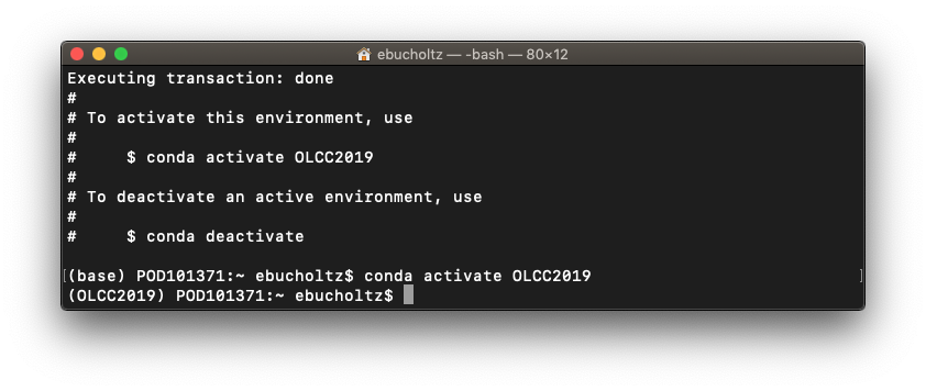
When you open your Ananconda prompt you will have something that looks like either:
| Windows | Mac |
 |
|
the (base) at the prompt indicates that you are in the base environment. We will be setting up our own environment for this course.
- Regardless of operating system use the package management system conda to create an enviornment called OLCC2019 using the version of python you just downloaded. To do so at the prompt type:
conda create -n OLCC2019 python=3.7
and follow any prompts to proceed with y. This will install install necessary packages.
- Regardless of operating system activate the environment. To do so at the prompt type:
conda activate OLCC2019
you should notice that the prompt no longer says base, but OLCC2019. To go back to the base, type conda deactivate. This will allow us to have multiple environments for this course if we need later.

- Regardless of operating system, install the following packages via conda. Each line below represents a command to type at the prompt.
Command What it does conda install -c conda-forge rdkit
Installs RDKit. The RDKit is an open source collection of cheminformatics and machine-learning software. conda install jupyter -y
Installs Jupyter notebooks. The Jupyter Notebook is an open-source web application that allows you to create and share documents that contain live code, equations, visualizations and narrative text. Uses include: data cleaning and transformation, numerical simulation, statistical modeling, data visualization, machine learning, and much more. conda install -c conda-forge scikit-learn -y
Installs Scikit-learn, which is a free machine learning software library for the python programming language. conda install -c conda-forge seaborn
the -y extension may not work with this command, so you will have answer y to proceed.Installs Seaborn, which is a Python data visualization library based on matplotlib. It provides a high-level interface for drawing attractive and informative statistical graphics. conda install -c mordred-descriptor mordred
Installs mordred, which is a Python library for a developed descriptor-calculation software application that can calculate more than 1800 two- and three-dimensional descriptors. conda install -c anaconda pip -y
Installs pip, which is the de facto standard package management system for python. conda install -c conda-forge pmw -y
Installs PyMol terminal window pop up within Jupyter Notebooks. pip install biopandas
Installs Biopandas which allows you to visualizemolecular structures of biological macromolecules (from PDB and MOL2 files) in pandas DataFrames. pip install pypdb
Installs PyPDB which is a python programming interface for the RCSB Protein Data Bank (PDB). Finally, lets do one more command to make sure all the conda installs have the proper updates and play well together:
conda update --all
You will have to click y to proceed.
This should be done as each package that was installed may be calling specifically for attributes that are in a previous version of a different package. Some packages may be updated, some new packages may be installed, and some packages may be downgraded. The goal is to create an environment where all packages play well together. - The final step is installation of pymol. Pymol is an open source molecular visualization system. Pymol has a paid version and a free version. The free version requires different installation steps dependent on the operating system you are using for this course.
Windows Mac - Download pre-compiled Open-Source PyMOL from Christoph Gohlke of the Laboratory for Fluorescence Dynamics, University of California, Irvine. There are lots of pre-compiled distributions. The filename you are looking for is:
pymol-2.4.0a0-cp37-cp37m-win_amd64.whl
\ \ \
\ \ \__ for 64 bit Windows
\ \
\ \___________ for Python 3.7.x
\
\__________________ PyMOL version 2.4.0a0 - Download the pre-compiled pymol lauchger as well:
pymol_launcher-2.1-cp37-cp37m-win_amd64.whl - In the conda OLCC2019 environment, switch to the download directory of your computer (e.g. C:\Downloads, or C:\Users\yourusername\Downloads) <
<OLCC2019> C:\> cd C:\Downloads
<OLCC2019> C:\> cd C:\Users\yourusername\Downloads
- Install the pymol launcher via pip (it also installs PyMol automatically)
pip install --no-index --find-links="%CD%" pymol_launcher-2.1-cp37-cp37m-win_amd64.whl
- Update Pymol with the following command:
pip install --upgrade --no-deps pymol-2.4.0a0-cp37-cp37m-win_amd64.whl
Mac install directions will be added later. If you are familiar with macports or homebrew these are the easiest ways to add.
- Download pre-compiled Open-Source PyMOL from Christoph Gohlke of the Laboratory for Fluorescence Dynamics, University of California, Irvine. There are lots of pre-compiled distributions. The filename you are looking for is:
- Link the conda environment to the Jupyter notebook.
python -m ipykernel install --user --name OLCC2019
- Start the jupyter notebook:
jupyter notebook
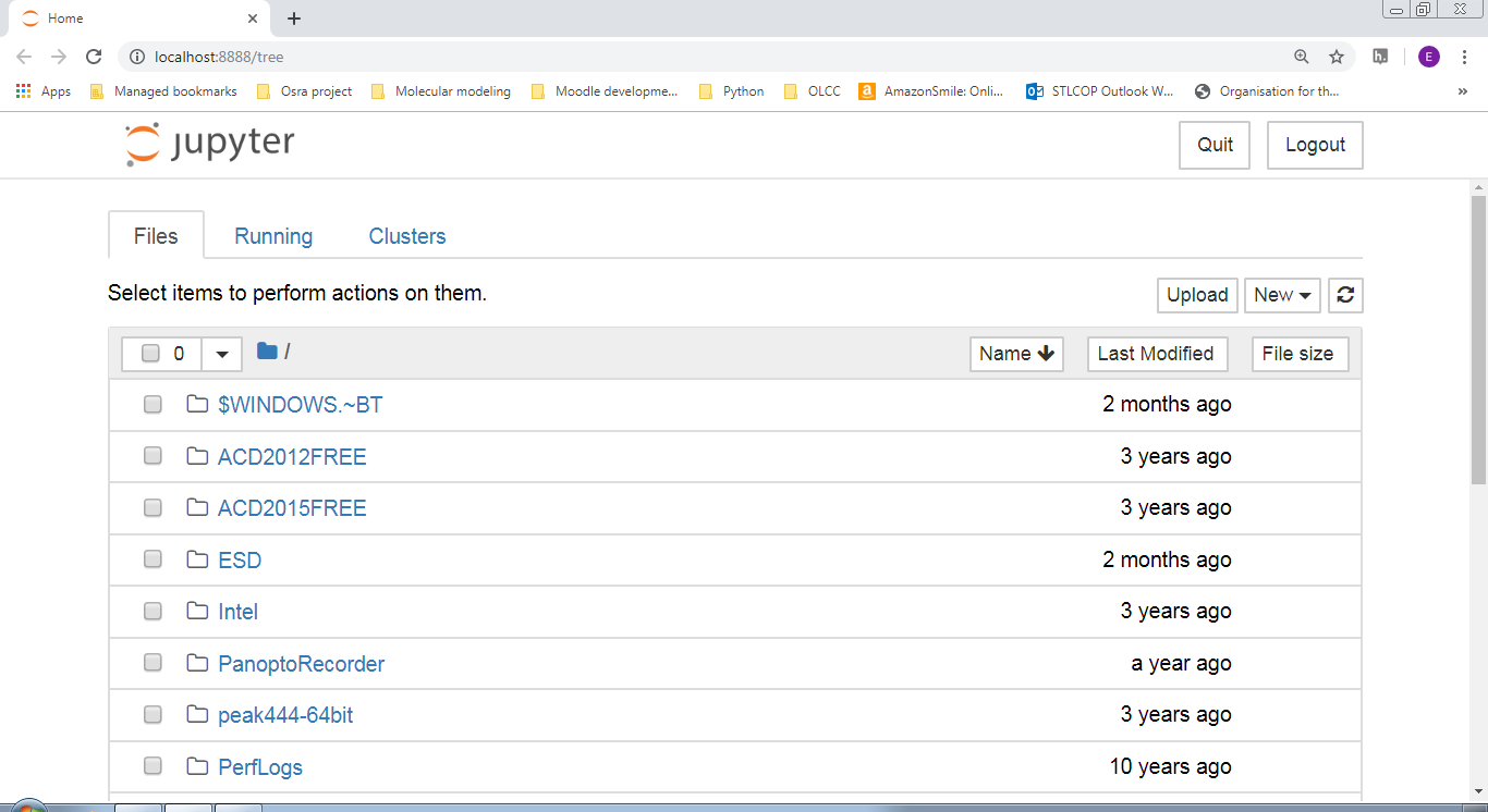
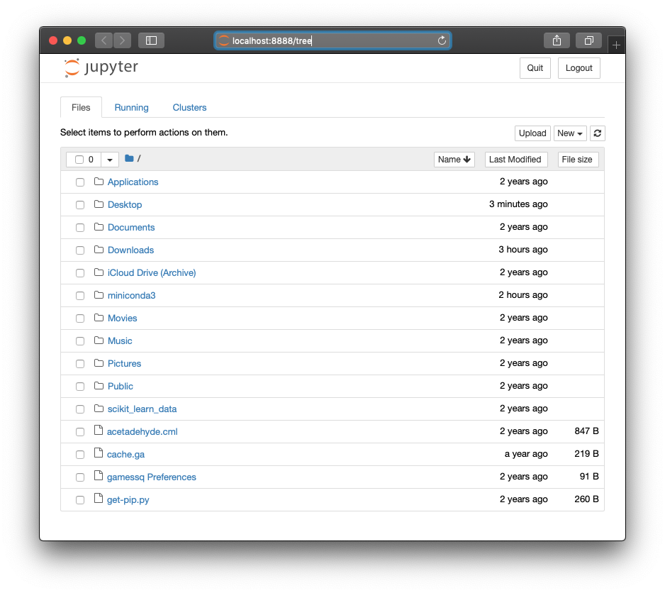
If you were successful, you should have a browser window that comes up like the following:
| Windows | Mac |
 |
 |
Notice that the website is running locally on your machine as localhost:8888/tree
You can save files, make new folders, change directors all from this window.


