11: Atomic Spectroscopy

The Hydrogen-Like Atom

A hydrogen-like atom is composed of a single electron and a nucleus with an arbitrary number of protons. In this laboratory the relationship between the wavelengths of light emitted from atoms and changes in quantum numbers will be explored.

Schrödinger’s equation in three dimensions is:

Equation (1)

\[\widehat{H}\psi =E\psi\] \[\widehat{H} =-\frac{\hbar^{2}}{2m}\nabla^{2}+V\left ( r,\theta, \varphi \right )\]
Where: \(\widehat{H}\) is the Hamiltonian, \(\psi\) is the wavefunction, E represents the possible energy levels, \(\hbar\) is Planck’s constant, h, divided by 2π, m is the particle’s mass. r, θ, φ are the spatial coordinates and V(r,θ,φ) is the potential energy.

A nucleus with an atomic number Z has a charge of Z_e where: e is the unit of elementary charge (the charge on a single proton or electron). Coulomb’s Law gives the force between an electron and the nucleus of an atom. Therefore the potential energy of an electron separated from the nucleus by a distance r is given by Equation (2) where ε_o is the vacuum permittivity:

Equation (2)

\[V=-\frac{Ze^{2}}{4\pi \epsilon _{o}r}\]

Equation (3) is Schrödinger equation for the internal motion of an electron relative to its nucleus.

Equation (3)

\[-\frac{\hbar^{2}}{2m}\nabla^{2}\psi -\frac{Ze^{2}}{4\pi \epsilon _{o}r}\psi=E\psi\] \[\mu = \frac{1}{m_{e}}+\frac{1}{m_{N}}\]

Where m_e is the mass of the electron and m_N is the mass of the nucleus.

The solution of Equation (3) yields the energy levels given by Equation (4).

Equation (4)

\[E_{n}=\frac{Z^{2}\mu e^{4}}{32\pi^{2}\epsilon _{o}^{2}\hbar^{2}n^{2}}\] if: \[R_{H}=\frac{\mu e^{4}}{32\pi^{2}\epsilon _{o}^{2}\hbar^{2}}\] Then: \[E_{n}=\frac{Z^{2}R_{H}}{ n^{2}}\]

R_H in Equation (4) is known as the Rydberg constant, R_H = 109,677 cm^-1. Energy levels for the hydrogen-like atom are plotted in Figure 1.


Figure 1. The energy levels of a hydrogen-like atom are shown compared with the energy levels of the particle in a box.

If an electron in an atom is excited to a higher energy level by passing an electric current a photon will be emitted when it falls to a lower energy level. The energy difference between the initial energy level and the final energy level is given by Equation (5). In Equation (5) n_f is the final energy level (lower energy) and n_i is the initial energy level (higher energy).

Equation (5)

\[E_{n}=Z^{2}R_{H}\left ( \frac{1}{n_{f}^{2}}-\frac{1}{n_{i}^{2}} \right ) \] or \[\frac{1}{\lambda _{n}}=Z^{2}R_{H}^{'}\left ( \frac{1}{n_{f}^{2}}-\frac{1}{n_{i}^{2}} \right )\]
A series of lines arises when electrons fall from higher energy levels to the same lower energy level, Figure 2. For the hydrogen atom when the final quantum number (n_f) is 1 you have the Lyman series, when n_f = 2 you have the Balmer series and when n_f = 3 you have the Paschen series. The series that you can see in the visible is the Balmer series.


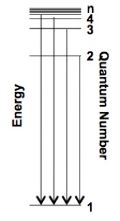
Figure 2. The Lyman Series is the series where n_f = 1, the excited electron falls into the ground state.

Procedure

1. Calculate the Rydberg constant in cm^-1 from the hydrogen lines in the Balmer series. These lines are the ones that you used in previous laboratories: 410.17, 434.05, 486.13 and 656.28 nm.

\[\frac{1}{\lambda \left ( cm \right )}=\frac{1}{\lambda (nm)\times 10^{7} cm }\]

• Note that the final quantum number for the Balmer series is 2. Therefore the initial quantum numbers must be greater than 2. The initial quantum numbers are 3, 4, 5 and 6. Match the initial quantum number with the correct emission above. To do this correctly think about which transition is the most energetic and with transition is the least.

• Now use Excel or similar application to plot \(\left ( \frac{1}{n_{f}^{2}}-\frac{1}{n_{i}^{2}} \right ) \); as the x-axis and \( \frac{1}{ \lambda_{n} (cm)} \); as the y-axis. You will get a very straight line.

• Determine the slope and intercept. The slope is the Rydberg constant. Note that it should be near R_H = 109,677 cm^-1.

2. Recalibrate your spectrometer using the calibration standard provided. The optical probe may be attached to the calibration standard by a screw fitting. The standard provides a mixture of Ar and Hg lines. The known wavelengths are given on the back of the calibration standard. Take a few spectra at different intensities. Make a new calibration curve using as many of the lines that you can identify from the calibration standard.

3. Take emission spectra of the Hg lamp at different intensities.

• Correct the measured emission line wavelengths of Hg using your new calibration curve.

• Convert the units of the emitted lines from wavelengths to cm^-1 by using Equation (6).

• Identify as many of the spectral lines as you can by using the NIST database at: http://physics.nist.gov/PhysRefData/ASD/index.html

4. Take emission spectra of the Ne lamp at different intensities. Repeat all of the steps in part 3 for Ne.

5. Take emission spectra of the Ar lamp at different intensities. Repeat all of the steps in part 3 for Ar.