Exact and Inexact Differentials
To study a system undergoing a change, we usually apply the principles of calculus; that is, we think of the overall change as occurring in a series of infinitesimally small steps. We must then ask ourselves if matters which small steps we take as we change the system.
If we can take any random assortment of small steps to make our change, and yet always get the same net change in the specific property we are studying, then that property is considered a state function. For a state function, each infinitesimal step that we add together by the process of integration is called an exact differential. When integrated, the sum of exact differentials is a value that is independent of path, depending only on the initial and final states. The change in internal energy is a state function, so the small steps involved in the change are exact differentials. In mathematical symbols, we can describe the change as
\[\int_i^f dU \, = \Delta U \, = U_f - U_i \label{2.4.1}\]
If the net change in the specific property we are studying depends on the specific path of small steps that we take, then that property is considered a path function. For a path function, each infinitesimal step that we add together by the process of integration is called an inexact differential. When integrated, the sum of inexact differentials is a value that is dependent of path, so the path between the initial and final states must be specified. The change in work is a path function, so the small steps involved in the change are inexact differentials. In mathematical symbols, we can describe the change as
\[\int_{i,path}^f dw \, = w \label{2.4.2}\]
It is important to note that we do not use the symbol \(\Delta w\) because \(w\) is not a state function, and the work that accompanies the change cannot be found from the simple calculation of \(w_f - w_1\).
Often we come to recognize or remember which properties are state functions and which are path functions. However, to help us identify which is which during calculations, it is useful to remember that a change in a state function can be symbolized by \(\Delta\), and that inexact differentials are often symbolized by using a "d" with a bar across the vertical line, đ.
Properties of Perfect Gases
In this section, we will look at a closed system (no matter can enter or leave, but energy can enter or leave) containing a sample of a perfect gas. The gas is described by the perfect gas law (PV = nRT), and because the system is closed, the only variables are V, T, and P. The internal energy of the gas can thus be described in terms of any two of these variables (because stating two of the variables automatically fixes the value of the third variable.)
The Internal Pressure, \(\pi_T \)
Internal pressure, \(\pi_T \), results from the interactions of the particles in a gas sample. An equation for internal pressure can be derived from the expression of internal energy as a function of volume and temperature:
\[dU = \left( \dfrac{\partial U}{\partial V} \right)_T \, dV \, + \, \left( \dfrac{\partial U}{\partial T} \right)_V \, dT \label{2.4.3}\]
As was shown in Topic 2.1, \(\left( \dfrac{\partial U}{\partial T} \right)_V \) is equal to the constant-volume heat capacity, \(C_V\). The first partial differential of Equation \(\ref{2.4.3}\), the internal pressure, is a measure of the change of internal energy of a sample as the volume changes under conditions of constant temperature. Thus,
\[\pi_T = \left( \dfrac{\partial U}{\partial V} \right)_T \label{2.4.4}\]
Equation \(\ref{2.4.3}\) can be rewritten as
\[dU = \pi_T \, dV + C_V \, dT \label{2.4.5}\]
If the gas is a perfect gas, there are no interactions among the particles in the sample and thus \(\pi_T \) = 0. In this case, the internal energy does not change as the space between the particles changes, and so internal energy is independent of the volume of the gas sample. For real gases, \(\pi_T \) may be greater than or less than 0, depending on whether attractive forces or repulsive forces among the particles dominate. If attractive forces in the gas sample are dominant, then \(\pi_T \) > 0, because as the particles are moved farther and farther apart, their potential energy increases. If repulsive forces in the sample are dominant, then \(\pi_T \) < 0, because the potential energy of the system decreases as the particles move farther apart.
The Expansion Coefficient, \(\alpha \)
The expansion coefficient \(\alpha \) is defined as the change in volume of a gas sample that occurs as the temperature increases under conditions of constant pressure. An expression for the expansion coefficient can be derived from Equation \(\ref {2.4.4}\) by first dividing both sides by dT:
\[\left( \dfrac{dU}{dT} \right) = \pi_T \left( \dfrac{dV}{dT} \right) + C_V \label{2.4.6}\]
Under conditions of constant pressure, the equation becomes
\[\left( \dfrac{\partial U}{\partial T} \right)_P = \pi_T \left( \dfrac{\partial V}{\partial T} \right)_P + C_V \label{2.4.7}\]
The expansion coefficient is related to the partial derivative \(\left( \dfrac{\partial V}{\partial T} \right)_P \), and is defined as
\[\alpha = \dfrac{1}{V} \left( \dfrac{\partial V}{\partial T} \right)_P \label{2.4.8}\]
The magnitude of \(\alpha\) is directly proportional to the extent of expansion of the gas sample as the temperature increases.
The Isothermal Compressibility, \(\kappa_T \)
The isothermal compressibility \(\kappa_T \) is a measure of the decrease in volume of a sample of gas that occurs as a result of an increase in pressure under conditions of constant temperature. The mathematical expression is
\[\kappa_T = - \dfrac{1}{V} \left( \dfrac{\partial V}{\partial P} \right)_T \label{2.4.9}\]
The negative sign is necessary to ensure that \(\kappa_T \) has a positive value because \(dV\) is always a negative value when the pressure is increased.
Example \(\PageIndex{1}\):
Determine the value of \(\kappa_T \) for an ideal gas.
Given: Equation \(\ref{2.4.9}\) and the relationship \(V = \dfrac{nRT}{P}\) for a perfect gas.
Solution:
\(\kappa_T = - \dfrac{1}{V} \left( \dfrac{\partial \dfrac{nRT}{P}}{\partial P} \right)_T = - \dfrac {1}{V} x \left( -\dfrac{nRT}{P^2} \right) = \dfrac{1}{V} x \dfrac{V}{P} = \dfrac{1}{P} \)
Exercise \(\PageIndex{1}\)
Determine the value of \(\alpha \) for an ideal gas.
Answer: \(\dfrac{1}{T}\)
The Relationship between \(C_V\) and \(C_P\) for a Perfect Gas
It is possible to derive a relationship between \(C_V\) and \(C_P\) for a perfect gas. We start with the previously derived relationships
\[C_P = \left( \dfrac{\partial H}{\partial T} \right)_P \label{2.4.10}\]
and
\[C_V = \left( \dfrac{\partial U}{\partial T} \right)_P \label{2.4.11}\]
Thus,
\[C_P - C_V = \left( \dfrac{\partial H}{\partial T} \right)_P - \left( \dfrac{\partial U}{\partial T} \right)_P \label{2.4.12}\]
If we recall that
\[H = U + PV = U + nRT \label{2.4.13}\]
then
\[C_P - C_V = \left( \dfrac{\partial (U + nRT)}{\partial T} \right)_P - \left( \dfrac{\partial U}{\partial T} \right)_P = nR \label{2.4.14}\]
The Relationship between \(C_V\) and \(C_P\) for a Real Gas
It is also possible to use \(\alpha\) and \(\kappa_T \) to derive a relationship between \(C_V\) and \(C_P\) for a real gas. We again start with the previously derived relationships
\[C_P = \left( \dfrac{\partial H}{\partial T} \right)_P \tag{2.4.10}\]
and
\[H = U + PV \tag{2.4.13}\]
then
\[C_P - C_V = \left( \dfrac{\partial H}{\partial T} \right)_P - C_V \label{2.4.15}\]
and
\[C_P - C_V = \left( \dfrac{\partial U}{\partial T} \right)_P + \left( \dfrac{\partial (PV)}{\partial T} \right)_P - C_V \label{2.4.16}\]
By substituting the definition of \(\alpha\) (Eqution \(\ref{2.4.8}\)) into Equation \(\ref{2.4.7}\) and rearranging, we get
\[\left( \dfrac{\partial U}{\partial T} \right)_P - C_V = \alpha \pi_T V \label{2.4.17}\]
Substituting Equation \(\ref{2.4.17}\) into Equation \(\ref{2.4.16}\) results in
\[C_P - C_V = \left( \dfrac{\partial (PV)}{\partial T} \right)_P + \alpha \pi_T V \label{2.4.18}\]
Again employing the definition of \(\alpha\) it can be shown that
\[\left( \dfrac{\partial (PV)}{\partial T} \right)_P = P \left( \dfrac{\partial V}{\partial T} \right)_P = \alpha PV \label{2.4.19}\]
which leads to
\[C_P - C_V = \alpha PV + \alpha \pi_T V \label{2.4.20}\]
The term \(\alpha PV\) represents the work done by the system to push back the atmosphere. The term \(\alpha \pi_T V \) represents the work required to break up the intermolecular forces of attraction among the particles of the sample.
It can be shown, using the second law of thermodynamics, that
\[\pi_T = T\left( \dfrac{\partial P}{\partial T} \right)_V - P \label{2.4.21}\]
Substitution of Equation \(\ref{2.4.21}\) into Equation \(\ref{2.4.20}\) leads to
\[C_P - C_V = \alpha TV\left( \dfrac{\partial P}{\partial T} \right)_V \label{2.4.22}\]
The partial derivative can be replaced by the following tactic
\[dV = \left( \dfrac{\partial V}{\partial T} \right)_P \, dT + \left( \dfrac{\partial V}{\partial P} \right)_T \, dP \label{2.4.23}\]
If \(\left( \dfrac{\partial (P)}{\partial T} \right)_V\) is at constant volume, then dV = 0 and Equation \(\ref{2.4.23}\) becomes
\[ \left( \dfrac{\partial V}{\partial T} \right)_P \, dT = - \left( \dfrac{\partial V}{\partial P} \right)_T \, dP \label{2.4.24}\]
Dividing by dT gives
\[ \left( \dfrac{\partial V}{\partial T} \right)_P = - \left( \dfrac{\partial V}{\partial P} \right)_T \left( \dfrac{\partial P}{\partial T} \right)_V \label{2.4.25}\]
which rearranges to be
\[\left( \dfrac{\partial P}{\partial T} \right)_V = - \dfrac{\left( \dfrac{\partial V}{\partial T} \right)_P}{\left( \dfrac{\partial V}{\partial P} \right)_T} \label{2.4.26}\]
Referring to Equations \(\ref{2.4.8}\) and \(\ref{2.4.9}\), it can be shown that
\[\dfrac{\alpha}{\kappa_T} = - \dfrac{\left( \dfrac{\partial V}{\partial T} \right)_P}{\left( \dfrac{\partial V}{\partial P} \right)_T} \label{2.4.27}\]
Thus, Equation \(\ref{2.4.22}\) becomes
\[C_P - C_V = \alpha TV\left( \dfrac{\partial P}{\partial T} \right)_V = \dfrac{\alpha^2 TV}{\kappa_T} \label{2.4.28}\]
This equation applies to all substances and phases. It collapses to equal \(nR\) for perfect gases, for which \(\alpha = \dfrac{1}{T}\) and \(\kappa_T = \dfrac{1}{P}\)
\[C_P - C_V = \dfrac{PV}{T} = nR \label{2.4.29}\]
The Joule-Thompson Effect
In 1852, working with William Thomson (who would later become Lord Kelvin), Joule conducted an experiment in which they pumped gas at a steady rate through a lead pipe that was cinched to create a construction. On the upstream side of the constriction, the gas was at a higher pressure than on the downstream side of the constriction. Also, the temperature of the gas was carefully monitored on either side of the construction. The cooling that they observed as the gas expanded from a high pressure region to a lower pressure region was extremely important and lead to a common design of modern refrigerators.
Not all gases undergo a cooling effect upon expansion. Some gases, such as hydrogen and helium, will experience a warming effect upon expansion under conditions near room temperature and pressure. The direction of temperature change can be determined by measuring the Joule-Thomson coefficient, \(\mu_{JT}\). This coefficient has the definition
\[ \mu_{JT} \equiv \left( \dfrac{\partial T}{\partial p} \right)_H \label{2.4.30}\]
Note: The derivation of \(\mu_{JT}\)
Referring to equation \(\ref{2.4.13}\), H = U +PV, we can say that
\[ dH = \left( \dfrac{\partial H}{\partial P} \right)_T dP ,\ + \left( \dfrac{\partial H}{\partial T} \right)_P dT \label{2.4.31}\]
Because the process is carried out at a constant enthalpy, dH =0. Thus
\[ 0 = \left( \dfrac{\partial H}{\partial P} \right)_T dP ,\ + \left( \dfrac{\partial H}{\partial T} \right)_P dT \label{2.4.32}\]
and
\[\left( \dfrac{\partial H}{\partial P} \right)_T dP = - \left( \dfrac{\partial H}{\partial T} \right)_P dT \label{2.4.33}\]
The partial derivative on the right side of equation \(\ref{2.4.33}\) is \(C_P\), so that
\[\left( \dfrac{\partial H}{\partial P} \right)_T dP = -C_P dT \label{2.4.34}\]
Dividing both sides by dP results in
\[\left( \dfrac{\partial H}{\partial P} \right)_T = - C_P \left( \dfrac{\partial T}{\partial P} \right)_H \label{2.4.35}\]
As defined in equation \(\ref{2.4.30}\), the partial derivative on the right side of equation \(\ref{2.4.35}\) is \(\mu_{JT}\):
\[\mu_{JT} = \left( \dfrac{\partial T}{\partial P} \right)_H \tag{2.4.30}\]
Thus for a closed system of constant composition under isenthalpic conditions,
\[dH = -\mu_{JT}C_P dP + C_P dT \label{2.4.36}\]
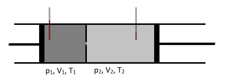
The following schematic shows how the Joule-Thomson coefficient can be measured by observing the temperature drop or increase a gas undergoes for a given pressure drop (Figure 2.4.1). The apparatus is thermally insulated so that no heat can be transferred in or out, making the expansion adiabatic.

Figure 2.4.1
Note: Why is the Process Isenthalpic?
The Joule-Thomson experiment is carried out adiabatically, so q = 0 and \(\delta U\) = w. The gas sample on the left is compressed isothermally under the constant pressure, \(P_1\). The volume of this gas changes from \(V_1\) to 0. Thus the work done on this gas is
\[ w_1 = -P_1 (0-V_1 ) = P_1 V_1 \label{2.4.37}\]
The gas on the right side of the equation expands isothermally (but possibly at a different constant temperature as the gas on the left) against the constant pressure, \(P_2\). The volume of this gas changes from 0 to \(V_2\). Thus the work done on this gas is
\[ w_2 = - P_2 (V_2 - 0) = - P_2 V_2 \label{2.4.38}\]
The total work done on the system of gases is
\[w_1 + w_2 = P_1V_1 - P_2V_2 \label{2.4.39}\]
Thus,
\[ \delta U = U_2 - U_1 = w_1 + w_2 = P_1V_1 - P_2V_2 \label{2.4.40}\]
which can be rearranged to the form
\[ U_2 + P_2V_2 = U_1 + P_1V_1 \label{2.4.41}\]
According to equation \(\ref{2.4.13}\), H = U + PV, so that equation \(\ref{2.4.41}\) can be simplified to
\[H_2 = H_1 \label{4.2.42}\]
In practice, the value of \(\mu_{JT}\) is difficult to obtain. Instead, the isothermal Joule-Thomson coefficient, \(\mu_T\), is obtained using an apparatus in which a gas at high pressure is passed through a porous plug into a lower pressure container. Because the gas will cool as it undergoes the pressure drop, heat is added to the gas after it has passed through the plug so that the gas remains at the same temperature on both sides of the pressure drop. \(\mu_T\) is the slope of the plot of enthalpy versus pressure at constant temperature:
\[\mu_T = \left( \dfrac{\partial H}{\partial P} \right)_T \label{2.4.43}\]
The value of \(\mu_T\) is converted to \(\mu_{JT}\) using the equation
\[\mu_T = - C_P \mu_{JT}\label{2.4.44}\]
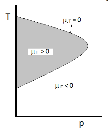
The typical behavior of the Joule-Thomson coefficient for a real gas can be summarized in Figure 2.4.2. At the combinations of T and p for which \(\mu_{JT} > 0\) (inside the shaded region), the sample will cool upon expansion. At those p and T conditions outside of the shaded region, where \(\mu_{JT} < 0\), the gas will undergo a temperature increase upon expansion. Along the boundary, a gas will undergo neither a temperature increase not decrease upon expansion. For a given pressure, there are typically two temperatures at which mJT changes sign. These are the upper and lower inversion temperatures.

Figure 2.4.2:
Using the tools of mathematics, it is possible to express the Joule-Thomson coefficient in terms of measurable properties. Consider enthalpy as a function of pressure and temperature: \(H(p, T)\). This suggests that the total differential \(dH\) can be expressed
\[dH= \left( \dfrac{\partial H}{\partial p} \right)_T dp+ \left( \dfrac{\partial H}{\partial T} \right)_p dT \label{totalH}\]
It will be shown later (again, once we develop the Maxwell Relations) that
\[\left( \dfrac{\partial H}{\partial p} \right)_T dp = -T \left( \dfrac{\partial V}{\partial T} \right)_p + V\]
A simple substitution shows
\[\left( \dfrac{\partial H}{\partial p} \right)_T dp = - TV \alpha + V = V(1-T\alpha)\]
So
\[ dH = V(1-T\alpha) dP + C_p dT\]
For an ideal gas, \(\alpha = 1/T\), so
\[ dH = \cancelto{0}{V(1-T\dfrac{1}{T}) dP} + C_p dT\]
which causes the first term to vanish. So for constant enthalpy expansion (\(dH = 0\)), there can be no change in temperature (\(dT = 0\)). This will mean that real gases show non-zero values for \(\mu_{JT}\) only because they deviate from ideal behavior!
Example \(\PageIndex{2}\):
Derive an expression for \(\mu_{JT}\) in terms of \(\alpha\), \(C_p\), \(V\), and \(T\).
Solution
Using the total differential for \(H(p, T)\) (Equation \ref{totalH}):
\[dH= \left( \dfrac{\partial H}{\partial p} \right)_T dp+ \left( \dfrac{\partial H}{\partial T} \right)_p dT\]
Dividing by \(dp\) and constraining to constant \(H\):
\[\left.\dfrac{dH}{dp} \right\rvert_{H}= \left( \dfrac{\partial H}{\partial p} \right)_T \left.\dfrac{dp}{dp} \right\rvert_{H} + \left( \dfrac{\partial H}{\partial T} \right)_p \left.\dfrac{dT}{dp} \right\rvert_{H}\]
Noting that
\[\left.\dfrac{dH}{dp} \right\rvert_{H} = 0\]
\[\left.\dfrac{dp}{dp} \right\rvert_{H} = 1\]
and
\[\left.\dfrac{dT}{dp} \right\rvert_{H} = \left(\dfrac{\partial T}{\partial p} \right)_{H}\]
so
\[ 0 = \left( \dfrac{\partial H}{\partial p} \right)_T + \left( \dfrac{\partial H}{\partial T} \right)_p \left(\dfrac{\partial T}{\partial p} \right)_{H}\]
We can then use the following substitutions:
\[\left( \dfrac{\partial H}{\partial p} \right)_T = V(1-T \alpha)\]
\[\left( \dfrac{\partial H}{\partial T} \right)_p = C_p\]
\[\left(\dfrac{\partial T}{\partial p} \right)_{H} - \mu_{JT}\]
To get
\[ 0 = V(1-T \alpha) + C_p \mu_{JT}\]
And solving for \(\mu_{JT}\) gives
\[\mu_{JT} = \dfrac{V}{C_p}(T \alpha -1)\]
A Molecular Explanation
When gas particles are allowed to expand into a volume of lower pressure, they are (obviously) likely to move father apart from each other than they originally were. If the pressure and temperature conditions are such that attractive intermolecular forces are dominant among the particles of the expanding gas sample, then the potential energy of these particles must be increased as they separate from each other. If the process is carried out under adiabatic conditions, the only source of energy is the kinetic energy of the particles themselves. Thus, as they move farther apart, their kinetic energy decreases, and therefore their temperature drops. When cooling occurs during expansion, we know that \(\mu_{JT}\) > 0.
It is also possible that the pressure and temperature conditions are such that repulsive intermolecular forces are dominant among the particles of the expanding gas sample, in which case the potential energy of these particles will be decreased as they separate from each other. If the process is carried out under adiabatic conditions, the only process by which the molecules can lose potential energy is to increase their own kinetic energy. Thus, as they move farther apart, their kinetic energy increases, and therefore their temperature increases. When heating occurs during expansion, we know that \(\mu_{JT}\) < 0.


