2.4: Accuracy and Precision

The information included in any quantitative measurement has two basic types of limitations or errors.

1. The first is accuracy. Even the best measuring devices are not perfectly accurate. For example, your bathroom scale at home may say that you weigh 197 lbs, but in fact, you weigh 199 lbs, your scale is reading incorrectly.
2. The second is precision. This is how well the information is known. Think about your bank account right now. How much information do you know? Do you roughly know the amount? Do you know the exact dollar amount? Do you know the cents? This limitation is the precision of your knowledge.

These two types of limitations will be further discussed below.

Precision and accuracy

A classic way to visualize the difference between precision and accuracy is to imagine throwing darts at a target, as illustrated in Fig. 2.4.1.

Figure \(\PageIndex{1}\): Representation of high accuracy with less precision (left) and low accuracy with high precision (right). Source: DarkEvil / Public domain

Systematic errors

Accuracy is effected by systematic errors. Systematic errors are constant, i.e., they have the same value in every measurement. For example, meter rod is a little short or a little long than a meter, it will introduce a systematic error. Systematic errors usually happen due to inaccurate calibration of the measuring instrument. The systematic errors determine how much the measured value differs from the actual value.

Random errors

Precision is effected by random errors. Random errors are the statistical variability of the measured number. Random errors vary from one observation to another. Random errors cancel out if many measurements are taken and averaged. Scientific measurements are usually taken at least in triplicate and averaged to minimize random errors. The random errors determine how close the repeat measured numbers are to each other.

Accuracy

Accuracy or trueness of the measurement is defined as how close the average value is to the actual value.

The closer the average is to the actual value, the more accurate or true it is, as illustrated in Fig. \(\PageIndex{1}\). The trueness depends on systematic errors, i.e., less systematic error, more accurate the average.

Precision

Precision is defined as how close the individual measurements are to each other.

The closer the individual values are to each other, the more precise the measurement is, irrespective of whether it is accurate or not, as illustrated in Fig. \(\PageIndex{1}\). Precision depends on random errors, i.e., more substantial random errors mean less precision.

Exact and inexact number

There are two types of numbers, count numbers that are exact and measured numbers that are inexact.

If the value is a counted number, it is an exact number.

That is, there is no error in it. For example, a purchase of one dozen oranges contains exactly 12 oranges; it can not be 11.5 or 12.5.

Inexact numbers and error range

When a value is measured, it comes with an error of measurement.

A measured number with an error is called an inexact number.

For example, when the same one dozen oranges are purchased by mass, the balance may read it 1572.6 g, or 1573 g, or 1570 g, depending on whether the smallest digit that the balance displays is 0.1g, 1 g, or 10 g. Suppose the balance is accurate to 1 g and reports the mass 1573 g; the actual mass may be anywhere in the range of 1572.5g-to-1573.4g. The smallest measured digit, i.e., the number in one's place, in this case, is an estimated number associated with an error. By convention, the estimated digit has ±1 errors associated with it. For example, the above-mentioned measured numbers are reported in science as 1572.6 g ± 0.1 g, 1573 g ± 1 g, or 1570 g ± 10 g, respectively. The estimated digits are shown in bold fonts in the examples.

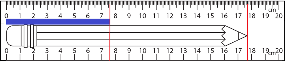
The smallest digit in the display of digital instruments is an estimated number. In measurement using instruments that do not have a digital display, the smallest digit marked on the instrument plus one digit less than the minimum marked digit is added to the reported value. The smallest reported digit is an estimated digit. For example, the length of the pencil in Fig 1.4.2 is reported as 17.7 cm using the ruler on the bottom, where 17 includes the smallest digit marked on the ruler, and the last digit, i.e., 0.7 is an estimated digit. By convention, the error range in this value is shown as 17.7 ± 0.1. The same length is 17.70 cm using the ruler on the top in Fig. 1.4.2l, where 17.7 includes the smallest digit marked on the ruler, and the last reported digit, i.e., 0, is an estimated digit. By convention, the error range in this value is shown as 17.70 ± 0.01. The estimated digits are marked in bold fonts.

Figure \(\PageIndex{2}\): Illustration of measurements that yield inexact numbers. The length of a blue rectangle is 7.60 ± 0.01 cm by using a more accurate ruler on the top and 7.6 ±0.1 cm by using a less accurate ruler on the bottom. The estimated digit is marked in bold fonts.