6.6: ICP-OES Operation Instructions

This page contains operating instructions for the Perkin Elmer Avio 220 Max at Duke Teaching Labs

I. Prepare the instrument and autosampler

1. Place the calibration solutions and the sample solutions in the auto sampler and record the position of each sample in your notebook. The auto sampler has a built in rack for ten 50 mL tubes (Positions 1-10) that are meant for standard solutions. In addition, there are three positions for removable sample racks that each accommodate 60 smaller, 15 mL tubes. Position 11 is in the back left corner of rack position R1, and the numbering of each row starts at the back of the autosampler rack (Figure \(\PageIndex{1}\)).

   

   Figure \(\PageIndex{1}\):The autosampler with rack positions labeled.

2. Check the rinse solution on the auto sampler. The two 2L carboys should be full of rinse solution (5% nitric acid) to ensure efficient rinsing. If the rinse containers are not filled, add dilute nitric acid solution to the 2L mark on each container. 
3. Check the waste container. If the container is fuller than the shoulders of the bottle, it should be emptied. Consult your instructor if the waste is full.
4. Adjust the peristolic pump tubing so that the pump moves liquid from the auto sampler into the nebulizer, and from the nebulizer drain into the waste. Ask your TA for help with this step.
5. Open the argon gas tank to 90 psi. Be sure there is sufficient pressure to operate the instrument. The ICP-OES instrument consumes argon at a rate of about 20 L/minute; one full compressed argon cylinder will provide about 6-8 hours of running time.
6. If you plan to measure absorbance below 190 nm, the optics should be purged with nitrogen gas and the compressed nitrogen tank should be opened.

II. Open the software 

1. Start the Synergistix for ICP Online instrument software by double clicking on the pink and purple "S" icon located on the desktop: 
    
2. At the top of the window, choose the Analysis tab. At the top of the Analysis tab menu, there are several tool boxes.

Note

There are two copies of the Synergistix for ICP instrument software on the computer. The "online" version directly controls the instrument and data collection. Methods and data cannot be manipulated in the "online" software while the instrument is actively collecting data or conducting performance checks. The "offline" version is meant for editing methods and performing data analysis without interfering with the "online" instrument operation.

III. Enter Sample Information

1. Go to the Sample Information tool box menu at the top of the main Analysis tab and choose New to create a new sample list.
2. Enter a file description. Then enter the auto sampler location (A/S Location) and sample information in the table. (enter only the samples, not the blanks or calibration standards).
   1. As you are entering the samples in this table, be sure to enter only the sample positions, and be sure to number then correctly. 
   2. If you are calibrating using the method of standard addition, please note that in the Autosample locations, each sample must be followed by its calibration standards, in consecutive order and increasing concentration of analyte. (see table with examples below) 
   3. Put all samples for your group in the sample tab see (below).  

   4. Example Sample locations for External calibration (samples can be in consecutive order).	Example Sample locations for Standard addition with five calibration solutions (samples cannot be in consecutive order).
      The image above is for an external calibration where the samples are in position 11,12,and 13. The locations of external calibration standards are set in the method editor.	The image above is for a 5 point calibration where the samples are in position 11,17,and 23. All intervening positions should contain the standard addition solutions for calibration.
      ...the method shown to the right would be appropriate for external calibration by simply uncheck the "Method of additions box" and leaving the A/S positions as they are.	...for a method of additions that looks like this (with 5 calibration solutions for each sample)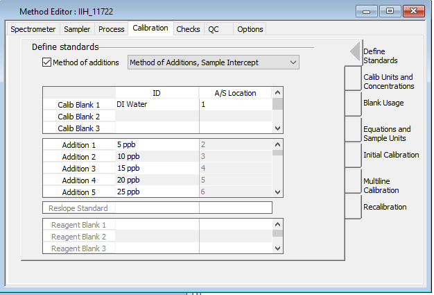

3. Save your sample list using the convention "YYYYMMDD_Qual_YOURINITIALS"  for qualitative analysis or "YYYYMMDD_Pb_YOURINITIALS" for quantitative analysis.

IV. Run the Calibration and Samples

Before proceeding, be sure your method and sample list are listed in the "Status" window on the right of the software window.

1. Go to the Analysis tab in the top menu and choose Analysis from the Analysis box. The Analysis window will open and it will use the current method and sample list to populate a "Run list". Check the list and be sure that the positions for each solution are correct.
2. Set a new file name under which to store your data under "Save data to Results Data Set". Use the same convention used for the method and sample list.

Using the scheduler to automatically shut down after an analysis.

To use the instrument overnight, make sure it is set up to turn itself off.

Go to Scheduler settings in the Analysis window or Scheduler under the Instrument tab. The following options will cause the instrument to completely shut down after the next analysis.

1. select shutdown
2. select at the end of automated analysis,
3. select including terminations caused by errors
4. select wash before shutdown for 1 minute
5. select turn off plasma and pump

Turn on the Plasma

The plasma should be turned on after you have set up everything else. This is to conserve argon gas, which is quite expensive and consumed quickly by the plasma.

1. Go to the Instrument Tab and select Plasma Control
2. In the Instrument Tab, use the menu at the top of the screen to do the following:
   1. Move the auto sampler to the wash location (if it is not already there).
   2. Turn the peristolic pump on. (Visually inspect to ensure the tubing is installed correctly and that it is pumping smoothly in the correct direction.)
   3. allow the wash solution to flow for at least 30 seconds.
   4. Move the sampling probe to a container with deionized water and flow for 30 seconds.
3. Open the Plasma Control from the Instrument tab, then press the plasma on/off button to turn the plasma on. If the instrument has not been used recently, the plasma may be unstable due to air being in the lines. If the plasma goes out soon after the first attempt at lighting, re-start the plasma after a few moments.
4. After a stable plasma is attained, check the nebulizer for proper operation. The easiest way to do this is to shine a bright light on the nebulizer and observe the mist that is created when the nebulizer is functioning properly.
5. choose the measure workspace ("ball menu" and select workspace--> measure) go to the Analysis tab to initiate analysis.

Run the list

After the plasma is on and stable, you have confirmed the instrument is performing as expected, and the run list has been generated, do the following.

1. Check again that the run list matches the locations of all solutions in the autosampler.
2. Check that the scheduler is set if you plan to run overnight.
3. Press "Analyze all" to initiate analysis of the solutiosn in the sample run list.

V. Manual operation

Manual operation is not typically used in the context of this course because it is more convinient to use the autosampler. 

Manual Calibration the instrument

1. Go to the Analyze tool box menu at the top of the main Analysis tab and choose Analysis.
   
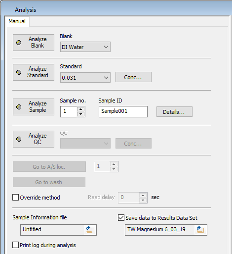
2. In the Analysis window, choose the Manual tab to open the Manual Analysis Control.
   (Or consult with your TA and decide whether if Automatic Analysis is a better option).
3. Change the name of the Results Data set to the format YYYYMMDDCHEM401L_YOURINITIALS.
   

4. Start the calibration with DI water.; this is the blank.  Go to the A/S location containing DI water using the "Go to A/S location" option in the Analysis window. Click on Analyze Blank in the Manual Analysis Control window to make the measurement.  The display in the Results window will show each of the three replicates and then report a mean, ABS(MEAN), standard deviation, SD, and relative standard deviation, RSD.  The instrument can auto zero the detector based on this blank if it is specified in your method.  You can watch the readings in real-time in the Results Tab, Spectra window.

5. Next, move the sample probe to the location of the least concentrated standard. Choose the correct standard in the dropdown menu and then click the Analyze Standard button in the Manual Analysis Control window to run the analysis of the standard solution.  Analyze the remaining standard solution from least-to-most concentrated in the same manner. (Give each group member a chance to operate the instrument.)

6. At the end of running your standards you have a graph of the absorbance vs concentration on the screen.  You have the regression statistics for the graph either at the bottom of the graph and/or in the Results window.  Export a pdf and an excel file of these results.

Manually Measure Samples

(If applicable)

Use the Analyze Sample button of the Manual Analysis Control window.  The ID for each sample was already specified in the Sample Information table (instructions above). Choose the sample for analysis and move the sample probe to the correct position. Then click the Analyze Sample button. Repeat for each sample. Aspirate deionized water when finished.

The results of the sample runs will automatically be saved in your data file.  You should print a pdf copy of the Results Window at the end of the run.  To "print" a pdf, click on the Results window to select it.  Next, click on the button at the top left of the main software screen and select Print Active Window.  Select CutePDF Writer from the list of available printers.  Save the pdf file and note the location where it is saved.  Feel free to create your own folder on the desktop where you can save all of your results over the two-week experiment.