3.4: UV-vis procedure and instructions for data analysis

Note: You should prepare a series of standard solutions of caffeine using serial dilution. You learned how to create serial dilutions in a previous module, and in this module you should come up with your own procedure for making the diluted series of solutions. Refer to Module 2 to review the correct use of volumetric glassware and determining error from a calibration curve. The solutions you make here will also be used in the HPLC module, so plan to store the solutions in sealed vials for later use.

Materials required:

• Caffeine (99%. powder)
• Ultrapure water
• Volumetric glassware
• Caffeine control solution (provided by TA and used in this module and the next)

Guidance for preparing the Standard Caffeine Samples

A. Prepare a stock solution of 0.1 g/L caffeine

1. Accurately weigh out 10.0 mg of caffeine. The caffeine can be found on the shelf near the weigh station area.
2. Transfer the caffeine into a clean 100 mL volumetric flask.
3. Dilute to the mark with deionized water. The stock solution will have a final concentration of 0.1 g/L.

Warning

There is a very small amount of caffeine powder, but it takes some time to dissolve completely. Be sure that caffeine is completely dissolved in about 50 mL of water before diluting to the volumetric mark and before proceeding to the next step. There is a sonicator in the lab that you can use to help break up small caffeine particles and aid in dissoltion.

B. Prepare a serial dilution

You should write out a specific plan for doing this before you get to lab (see pre-lab assignment). Carry out a serial dilution to obtain a series of standard solutions that are are approximately evenly spaced (in terms of their concentrations). The highest concentration should be about \(0.05 \pm 0.1\) g/L, and the lowest concentration solution should be approximately \(0.005 \pm 0.005\). Make enough of each solution so that you have at least 10 mL of each solution to play with. You should use ultrapure deionized water to make all solutions and dilutions. Ensure adequate mixing in each diluted solution before using it to create the next.

Tips

You have access to:

• volumetric flasks to contain of 5, 10, 25, 50, 100, 250, 500, and 1000 mL
• volumetric pipete to deliver volumes of 1, 2, 3, 4, 5, 10, 15, 20, 25, 50, and 100 mL
• automatic pipetters to deliver between 100-5000 mL

When an experienced student did this lab, she used only one 25 mL volumetric flask, one 10 mL volumetric pipette to create a series of solutions. 

**Do not discard your solutions. Save the solutions for the next module!

Procedure for analysis of caffeine with UV-vis and validating solution concentrations

Start up:

At the begriming of the lab period, check to confirm that the UV-vis is switched "on". The Cary 100 instruments have tungsten and deuterium lamps that must be warmed up for approximately 1 hour prior to use. The Cary 60 instrument has a xenon flash lamp, which does not require warm up. Be sure you discuss which instrument you will use with your TA, and if you are using a Cary 100, be sure it is on for 1 hour prior to use.

Validate instrument:

Prior to using any instrument, you should run checks to ensure the instrument is functioning properly. While the Cary UV-vis instruments run initialization procedures upon startup, there is a "Validate" program that will validate the instrument's performance. You should run a wavelength validation after the instrument has warmed up (if applicable). For Cary 100 instruments, use the deuterium (D2) lamp to validate wavelength accuracy. For the Cary 60, use the tungsten (W) lamp to calibrate wavelength accuracy. The figure below gives a summary of the steps involved in validating the instrument.

1. Find the "Cary WinUV" shortcut on the computer desktop and open it. The linked folder contains all the programs that operate the Cary spectrophotometer. Open the "Validate" Program.
   • The Validate window should open. At the top left corner of the window, it should say "Validate-Online". If it says otherwise (ie "Validate-Offline, as pictured below) then it is not connected to the instrument. Wait a few moments to see if it connects. In the meantime, make sure the instrument is powered on. If it does not connect, try pressing "connect" (its where the start button is), and if that fails, get help.
2. On the left hand side of the Validate Window, choose "Tests".
   • The Tests window will open. Choose "Instrument Performance Tests".
   • There should be a list of several available tests in the "Test Order" box. If there is not, double check that the instrument is "online". Then, press the "Reset all limits to Default button" - this usually regenerated the list of available tests.
3. It is sufficient to run one wavelength validation test. In the "Test Order" box, choose the wavelength accuracy test that uses the instrument's own lamp (either D2 or W). To do this, you should remove all other tests by selecting each and pressing the "remove test" button that is just to the right of the box (it looks like an exclamatino point with a red "X". Do this until the test you want is the only one remaining.
4. Press "OK" after you have specified the validation test to be run.
   • The USP Tests box will close.
5. Check to make sure there are no samples in the light path. Close the sample compartment. Then Press "Start".
   • This should initiate data collection. It will take a few minutes, and during this time you should be able to see the collected spectrum recorded on the screen. If not, get help.

Figure \(\PageIndex{1}\): A visual summary of steps involved in validating the Agilent Cary UV-vis spectrophotometers. (CC-BY-NC-SA; Kathryn Haas)

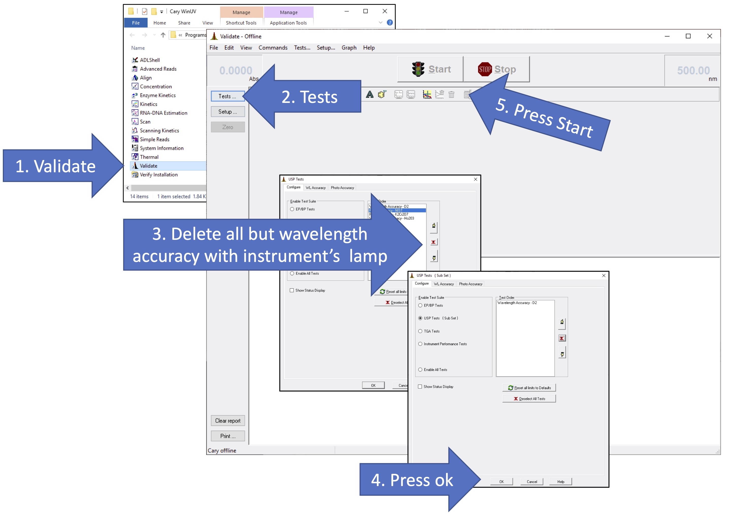
After the validation, copy and paste the relevant data and images from the report into your ELN.

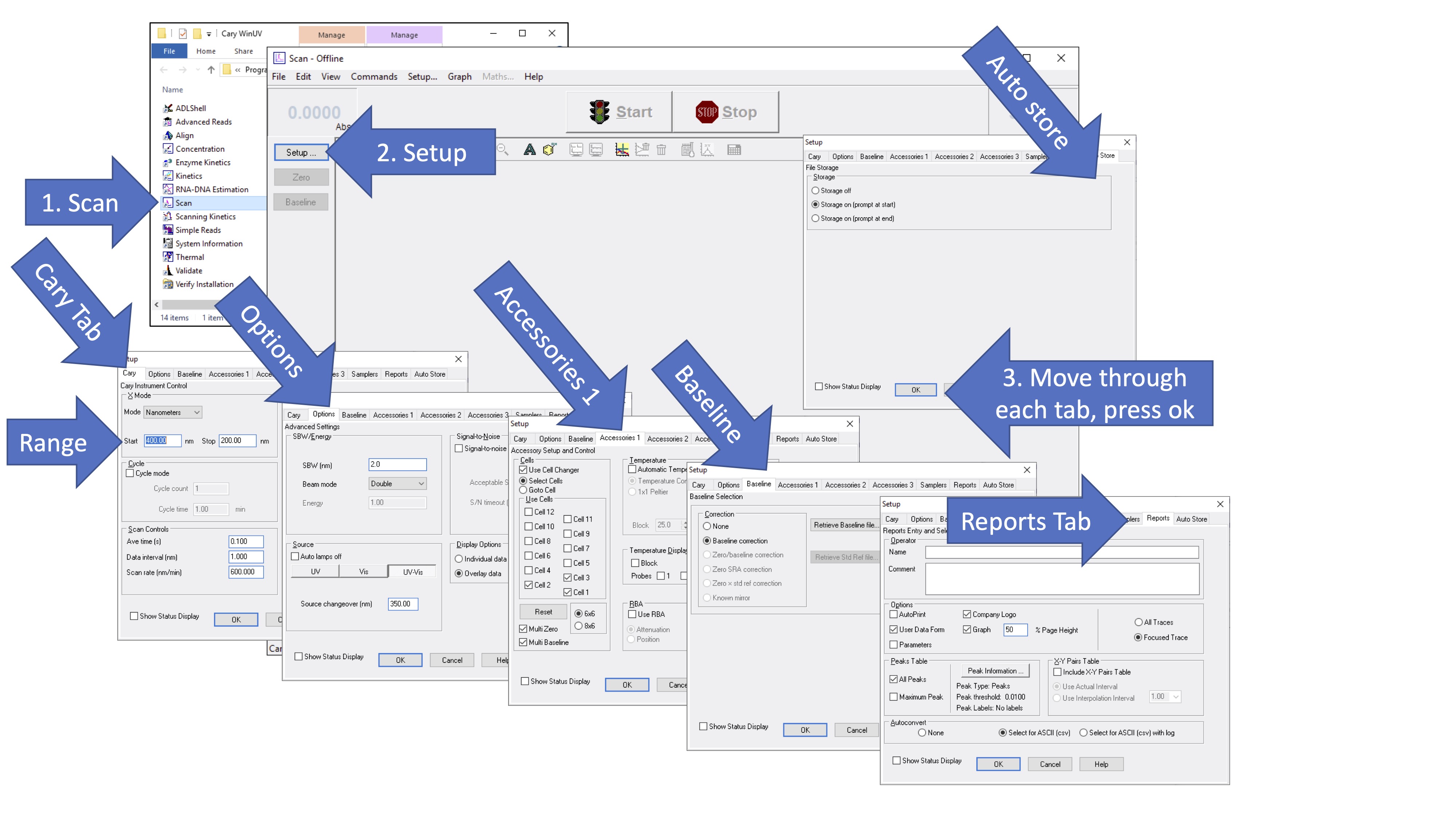
Settings:

Open the "Scan" program on the Cary UV-vis and got to "Settings". Go to each tab and modify the settings in the following order.

• Cary Tab:
  • Set the scan range to include wavelengths of 400-200 nm (or a wider range if you prefer).
  • Set the data interval to 1 nm and the average time to 0.1 s.
• Options:
  • SBW/Energy: Use double beam mode
  • Source: Choose either UV or UV-vis 
  • Display Options: Choose "Overlay Data"
• Accessories 1: This is the multi-cell, temperature-controlled sample holder. If this accessory is attached, follow the instructions below. Otherwise, uncheck the "Use cell changer" option.
  • If the multi-cell changer is installed, select "Use cell changer". Note that the cell changer must be installed correctly and aligned to operate correctly.
  • Check only the cell poisitions that you will use during the experiment.
  • Select multi-zero
  • Select multi-baseline
• Baseline:
  • Select Baseline correction
• Reports:
  • Select for ASCII (csv). This option saves the data as a comma delineated format that can be opened in excel or and plotted using your own computer.
• Auto Store:
  • "Storage on (prompt at start)" should be selected

The figure below gives a visual summary of the stesp above. After all settings have been chosen, press "OK". The instrument is ready for you to use at this point.

Figure \(\PageIndex{2}\): A visual summary of steps involved in setting up the Scan application for the Agilent Cary UV-vis spectrophotometers. (CC-BY-NC-SA; Kathryn Haas)

Data collection:

Depending on the sample holder and the number of samples you plan to run, the procedure below could vary slightly. Make sure to consult your instructors about any changes to this procedure.

1. Use the Scan program to collect a baseline spectrum. You will need either one or two cuvettes containing a sample blank (ie no analyte). The cuvette should not be empty - rather it should contain the background solution of your sample, but with no analyte. (In the case here, it should be ultrapure water). Put the cuvette with a blank solution into the appropriate position(s) to baseline the instrument. Then press the "Baseline" button on the left of the Scan window.
2. Place sample in the appropriate position(s) and press "Start".
3. Specify the file name and folder location where the data should be saved.
   • All data should be saved in the directory C:\Data\CHEM401L\ within a folder for your group. Make a new folder within the CHEM401L directory if one does not already exist.
   • Your file names should follow the convention "YYYYMMDD_Initials_##". In your notebook, you should keep a log of file names and a description of what is contained in each file. Prepare a table in your notebook for recording this information. Example is below (this info is made up!):

     File Location is C:\Data\CHEM401L\OurGroup File Names: 20230811_KH_##	Absorbance at \(\Lambda_{max}\)	Solution components	Comments
     20230811_KH_01	0.0001	ultrapure water	This was take just to check that the blank is as expected (ie a flat line)
     20230811_KH_02	0.0809	0.01 g/L caffeine in ultrapure water
     20230811_KH_03

4. Repeat the steps above for each calibration solution and the control solution. If you use the same cuvette for each, you do not need to repeat the baseline step. However, you should ensure that your spectrum is at zero absorbance near 400 nm. If not, check with your instructors.
5. After you have collected each all data, it is helpful if you "save as" all of your data in one "bulk" .csv file. To do this, choose "file" and then "save as" and choose ".csv". Give the file a name like "YYYYMMDD_Initials_all" to indicate it has "all" your data. Open this file using excel and check that it in fact contains all the spectra that you collected.

Data Transfer:

Before you start cleaning up, check to be sure that you can find your data, and that they are in fact saved as .csv files. Transfer your data files to your own computer (email is fine, or use OneDrive or Box).

Check following:

1. You have YOUR data (not someone else's)
2. You can open the files on your computer
3. You know what is in the files and how they are structured
4. You have a plan for how to plot the spectra and create the calibration curve from the data

Treatment of Data

The following should be prepared prior to moving forward with the next module. These items should be checked by your instructors, and you should plan to include them in your caffeine analysis report. (Note that the report encompasses this module and the next on HPLC)

• A figure containing overlaid spectra collected for the calibration curve, with wavelength of maximum absorbance indicated on the plot. This figure should include all the necessary labels and formatting that was required of previous figures/plots. Include title, labels with units, annotations, a figure number and a descriptive caption. Include a legend and choose a line type and color scheme that is legible to a reader who is colorblind.
  • This figure could be generated using the Scan software or by plotting with MatLab or other plotting program.
• A plot of the calibration curve with best fit line and "the works" (ie everything that is expected of such a plot and its accoutrements - see the previous module for expectations on such a plot).
• Validation of the calibration curve including error analysis and comparison to a control solution.
  • This should be used as evidence that your solutions have been prepared correctly and that the concentrations are as expected.
  • If you cannot validate your calibration curve, use the molar extinction coefficinet for caffeine reported in a reputable peer-reviewd journal to determine the actual concentrations of caffeine in your solutions, and explain why they are different than the expected concentrations.