5.2.1: The Electromagnetic Spectrum and Molecular Transitions

 

Electromagnetic radiation, or light, exhibits dual behavior as both waves and particles. Wave properties, such as refraction, best explain phenomena like light passing through different mediums. Conversely, particle behavior provides a more accurate description in certain scenarios, like absorption and emission. The nature of electromagnetic radiation remains unclear, with wave and particle models coexisting since the development of quantum mechanics in the early 20th century. Despite this ambiguity, these dual models effectively characterize electromagnetic radiation.

It consists of oscillating electric and magnetic fields that travel through space at a constant velocity. In a vacuum, the speed of light (c) is \(2.99792 \times 10^8 \frac{m}{s}\). When passing through a medium other than a vacuum, its velocity (v) is slightly less than c, with the difference being <0.1%. For practical purposes, the speed of light is often approximated as \(3.00 \times 10^8 \frac{m}{s}\). The oscillations in the electric and magnetic fields are perpendicular to each other and the wave's propagation direction. An model of plane-polarized electromagnetic radiation, featuring a single oscillating electric field and a single oscillating magnetic field, is illustrated in Figure \(\PageIndex{1}\).

Figure \(\PageIndex{1}\): Plane-polarized electromagnetic radiation showing the oscillating electric field in red and the oscillating magnetic field in blue. The radiation’s amplitude, A, and its wavelength, λ, are shown. Normally, electromagnetic radiation is unpolarized, with oscillating electric and magnetic fields present in all possible planes perpendicular to the direction of propagation.

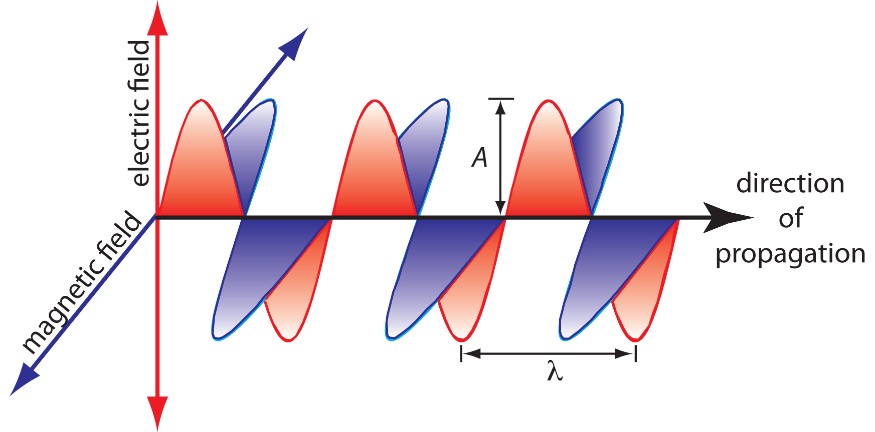
An electromagnetic wave is characterized by several fundamental properties, including its velocity, amplitude, frequency, phase angle, polarization, and direction of propagation. For example, the amplitude of the oscillating electric field at any point along the propagating wave is

\[A_\ce{t} = A_\ce{e}\sin(2π \nu t + \phi)\]

where \(A_\ce{t}\) is the magnitude of the electric field at time \(t\), \(A_\ce{t}\) is the electric field’s maximum amplitude, \(\nu\) is the wave’s frequency—the number of oscillations in the electric field per unit time—and \(\phi\) is a phase angle, which accounts for the fact that A_t need not have a value of zero at t = 0. The identical equation for the magnetic field is

\[A_\ce{t} =A_\ce{m}\sin(2π \nu t + \phi)\]

where A_m is the magnetic field’s maximum amplitude.

Units of energy

The wavelength, λ, is defined as the distance between successive maxima (Figure \(\PageIndex{1}\)). The relationship between wavelength (in m) and frequency (in \(s^{-1}\) or \(Hz\)) is given below. Wavelength is usually expressed in nanometers (1 nm = 10^–9 m) for ultraviolet and visible light, and in microns (1 μm = 10^–6 m) for infrared light.

\[λ = \dfrac{c}{\nu}\ \label{eq1}\]

Wavelength is a unit used often by chemists, especially in UV-vis spectroscopy. Because it is inversely related to energy (ie smaller wavelengths are higher energy), many scientists prefer units that are directly proportional to energy. An alternate unit, the wavenumber, \(\tilde{ν}\), is used frequently, especially in infrared spectroscopy. In general it seems to be the preferred unit of physicist due to its direct correlation to energy. It is useful to know how to convert between these two commonly-used units. The unit \(\tilde{ν}\) is simply the reciprocal of wavelength.

\[\tilde{ν} = \dfrac{1}{λ} \label{eq2}\]

Wavenumbers are frequently used to characterize infrared radiation, with the units given in cm^–1.

Keeping symbols straight

Heads up! The word "frequency" refers to cycles per unit time, but can also be measures in a length scale. Frequency measured in cycles per seconds (\(s^{-1}\) can be expressed in the metric base unit Hertz, and can have the symbol \(f\) or \(\nu\). When it is expressed in a length scale, like wavenmumbers (\(cm^{-1}\), it has the symbol \(\tilde{\nu}\). 

When converting units from \(\nu\) (in \(s^{-1}\)) to \(\lambda\), use the speed of light to convert between time and length scales as in \ref{eq1}. When converting from \(\tilde{\nu}\) to \(\lambda\), use \ref{eq2} and convert metric units as necessary.

Regions of the Spectrum and Types of Transitions

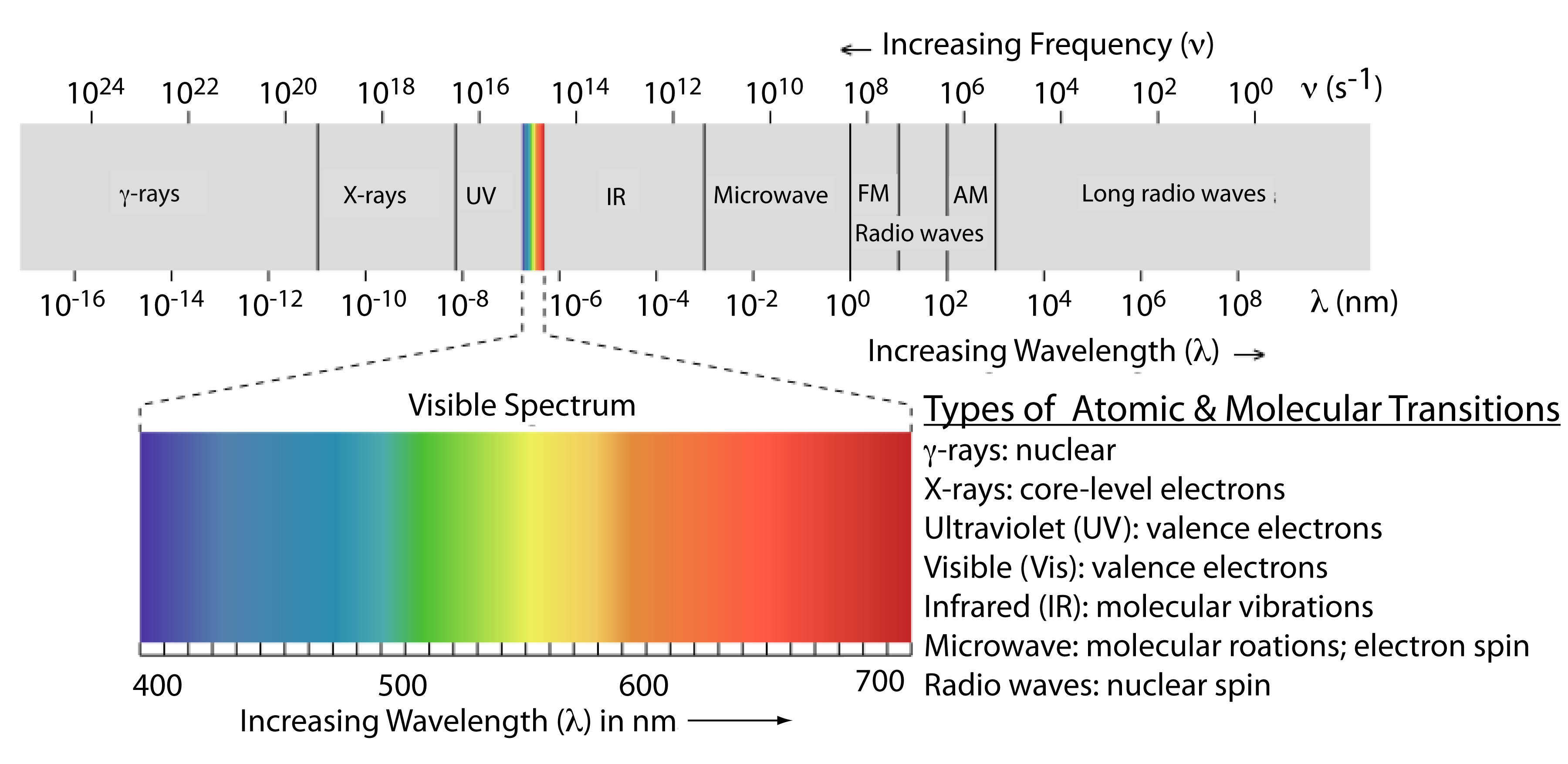
Electromagnetic radiation spans a wide range of frequencies and wavelengths, prompting the division of this spectrum into distinct regions for convenience, known as the electromagnetic spectrum (Figure \(\PageIndex2\)). These divisions are based on the atomic or molecular transitions responsible for the absorption or emission of photons. It's important to note that the boundaries between these regions are not fixed, allowing for potential overlap between different spectral regions.

Figure \(\PageIndex{2}\): The electromagnetic spectrum showing the boundaries between different regions and the type of atomic or molecular transition responsible for the change in energy. The colored inset shows the visible spectrum. Source: modified from Zedh (www.commons.Wikipedia.org).

Given the energy levels of molecules and their corresponding wavelengths, we can determine the frequency within the electromagnetic spectrum regions using the equation:

\(\Delta E=E_u-E_l=h\)

Here, \(h\) represents the energy change between the upper (\(u\)) and lower (\(l\)) states.

The frequencies of molecular transitions fall within specific ranges. These ranges are listed in the table below in order of increasing energies.

Wavelengths	Frequency (\(cm^{-1}\))	Frequency (s^-1)	Region	Transitions
1 mm - 1 m	~ 0.01	10^8 - 10^11	microwave	rotational transitions of large polyatomic molecules
~100 \(\mu\)m	~10	10^12	far infrared	rotational transitions of small molecules
~ 10 \(\mu\)m	~100 - 5000	~ 10^13	infrared	vibrational transitions
~700 - 400 nm	~ 14,000 - 25,000	~10^14	visible and ultraviolet	electronic transitions

 

Absorption and Emission

In absorption spectroscopy a photon is absorbed by an atom or molecule, which undergoes a transition from a lower-energy state to a higher-energy, or excited state (Figure \(\PageIndex{3}\)). The type of transition depends on the photon’s energy (see table above). Absorbing electromagnetic radiation can cause transitisions (excitations) in the rotational, vibrational, or electronic states depending on the energy of the photon. Likewise, relaxation of the molecule back to a lower-energy rotational, vibrational, or electronic state can result in emission of a photon (Figure (\PageIndex{3}\)). 

Figure \(\PageIndex{3}\): Simplified energy diagram showing the absorption and emission of a photon by an atom or a molecule. When a photon of energy hν strikes the atom or molecule, absorption may occur if the difference in energy, ∆E, between the ground state and the excited state is equal to the photon’s energy. An atom or molecule in an excited state may emit a photon and return to the ground state. The photon’s energy, hν, equals the difference in energy, ∆E, between the two states.

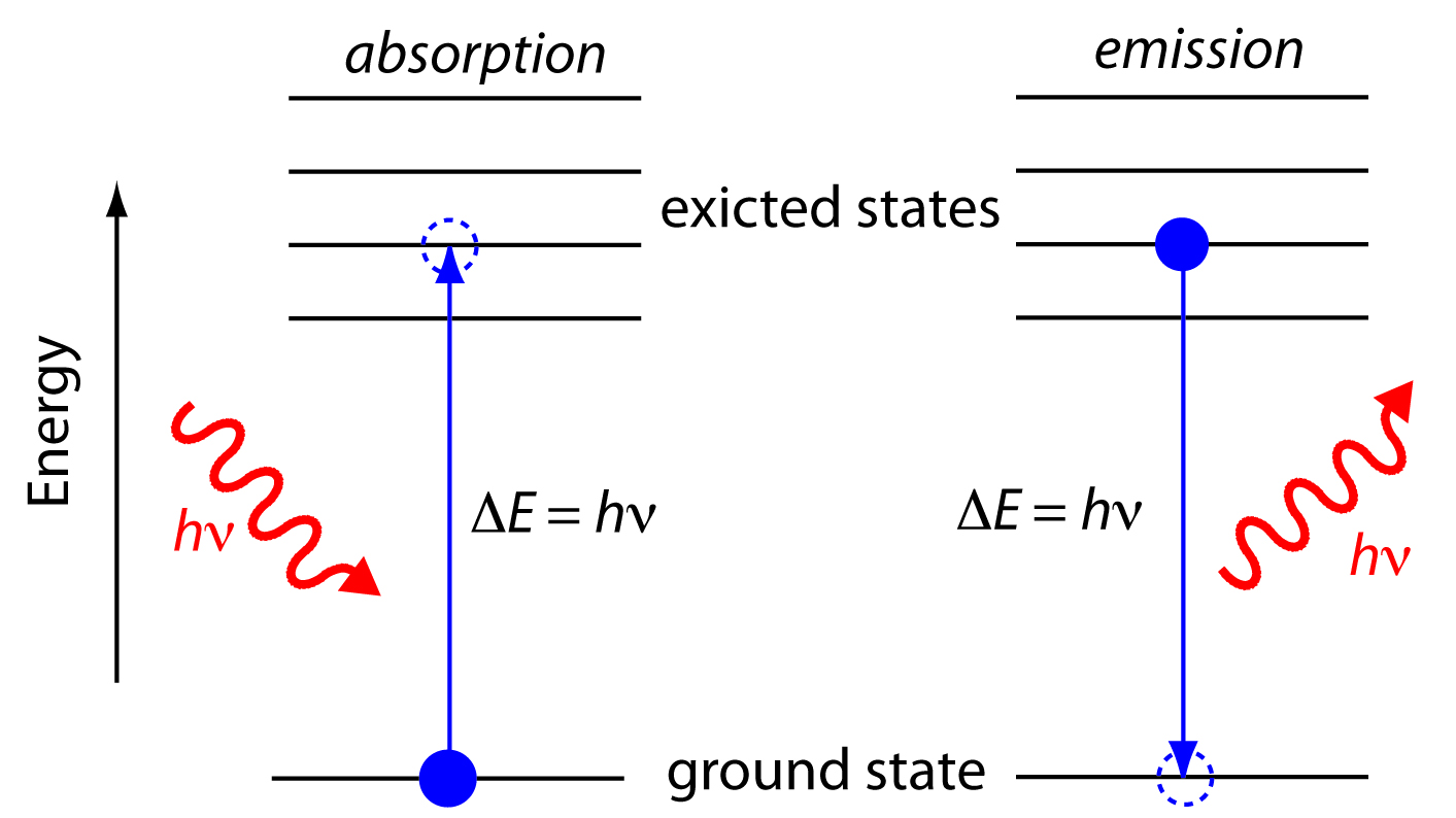
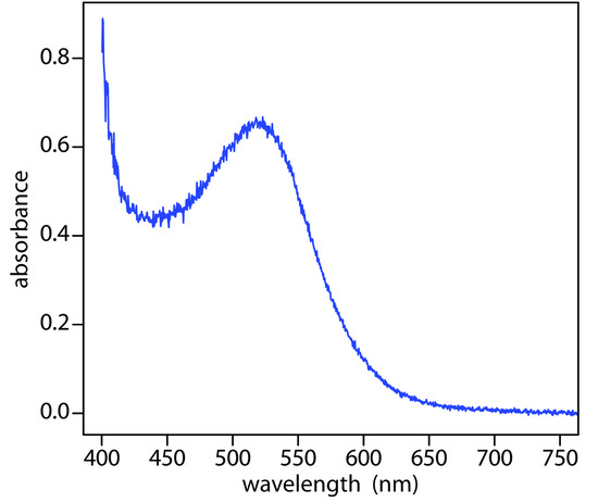
When it absorbs electromagnetic radiation the number of photons passing through a sample decreases. The measurement of this decrease in photons, which we call absorbance, is a useful analytical signal. Note that each of the energy levels in Figure \(\PageIndex{3}\) has a well-defined value because they are quantized. Absorption occurs only when the photon’s energy, hν, matches the difference in energy, ∆E, between two energy levels. A plot of absorbance as a function of the photon’s energy is called an absorbance spectrum. Figure \(\PageIndex{4}\), for example, shows the visible absorbance spectrum of cranberry juice.

Figure \(\PageIndex{3}\)). Visible absorbance spectrum of cranberry juice. As a result, the juice appears red.

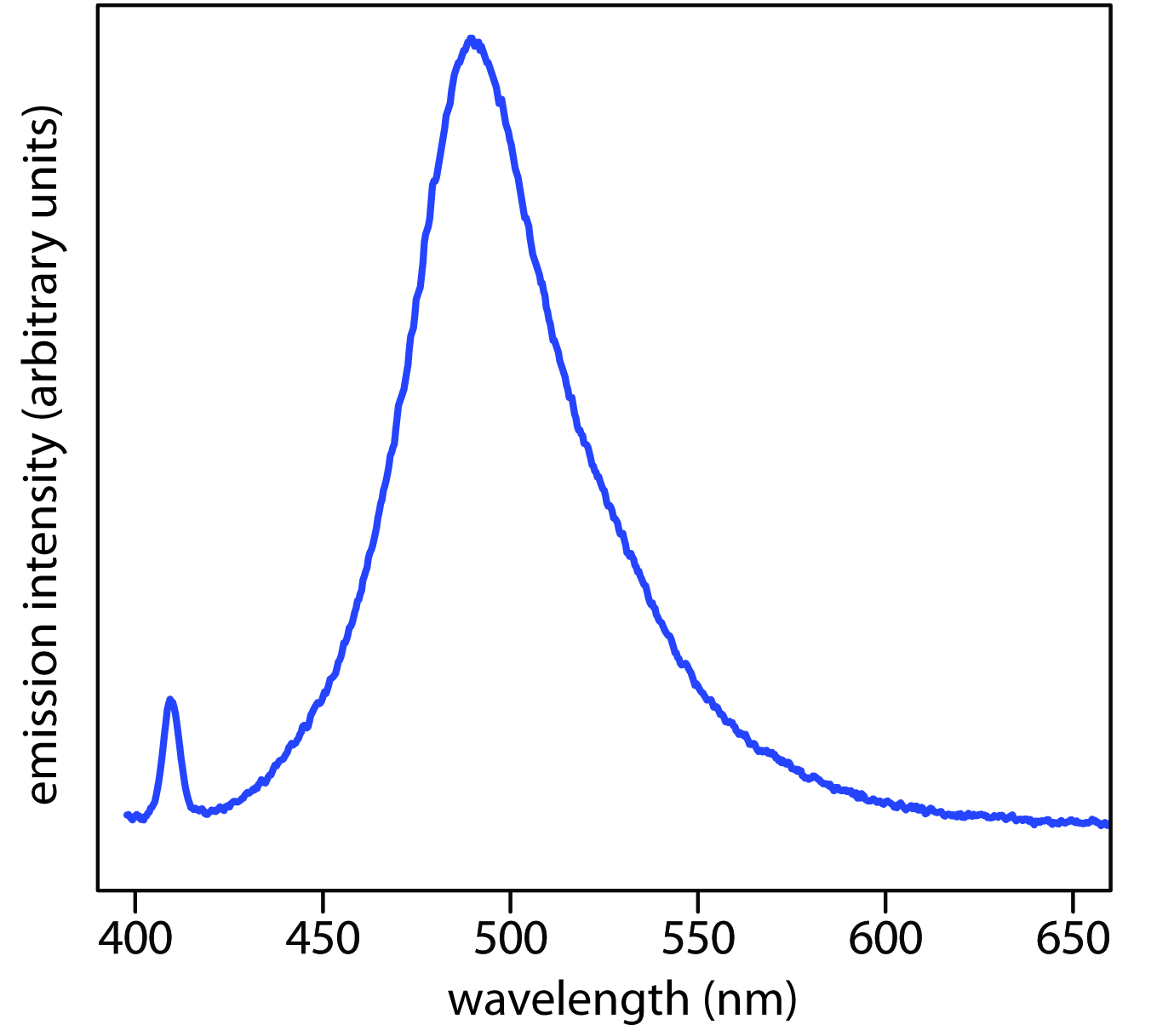
When an atom or molecule in an excited state returns to a lower energy state, the excess energy often is released as a photon, a process we call emission (Figure \(\PageIndex{4}\)). There are several ways in which an atom or molecule may end up in an excited state, including thermal energy, absorption of a photon, or by a chemical reaction. Emission following the absorption of a photon is also called photoluminescence, and that following a chemical reaction is called chemiluminescence. A typical emission spectrum is shown in Figure \(\PageIndex{5}\).

Figure \(\PageIndex{5}\): Photoluminescence spectrum of the dye coumarin 343, which is incorporated in a reverse micelle suspended in cyclohexanol. The dye’s absorbance spectrum (not shown) has a broad peak around 400 nm. The sharp peak at 409 nm is from the laser source used to excite coumarin 343. The broad band centered at approximately 500 nm is the dye’s emission band. Because the dye absorbs blue light, a solution of coumarin 343 appears yellow in the absence of photoluminescence. Its photoluminescent emission is blue-green. Source: data from Bridget Gourley, Department of Chemistry & Biochemistry, DePauw University).

Contributors and Attributions

• Jim Clark (Chemguide.co.uk)

• • Gamini Gunawardena from the OChemPal site (Utah Valley University)

• David Harvey (DePauw University)