9.5: Transcriptomics
- Page ID
- 347471
Consider a matrix containing all of the known gene sequences in a genome. To make such a matrix for analysis, one would need to make copies of every gene, either by chemical synthesis or by using the polymerase chain reaction. The strands of the resulting DNAs would then be separated to obtain single-stranded sequences that could be attached to the chip. Each box of the grid would contain sequence from one gene. With this grid, one could analyze the transcriptome - all of the mRNAs being made in selected cells at a given time. For a simple analysis, one could take a tissue (say liver) and extract all the mRNAs from it. This mRNA population represents all the genes that were being expressed in the liver cells at the time the RNA was extracted. These RNAs should be able to hybridize (base-pair) with their corresponding genes on the microarray. Genes that were not being expressed would have no mRNAs to bind to their corresponding genes on the grid.

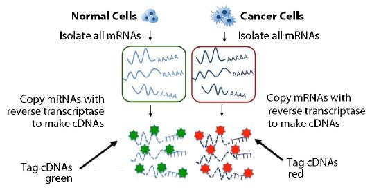
Figure 8.25 - Copying and labeling of transcriptome. Image by Taralyn Tan
In practice, the mRNAs are not used directly, but are copied into single-stranded DNA copies called cDNAs. The cDNAs are tagged with a fluorescent dye and added to the microarray under conditions that allow base pairing so that the cDNAs can find and base pair with complementary sequences on the matrix (Figure 8.26). The matrix is then washed to remove unhybridized cDNAs. The presence/absence/abundance of each mRNA is then readily determined by measuring the amount of dye at each box of the grid.
Figure 8.26 - Add labeled cDNAs to microarray plate. Image by Taralyn Tan
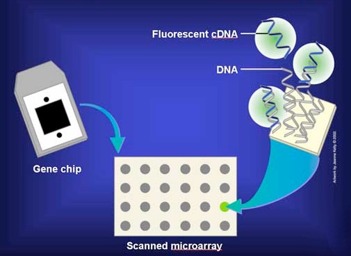
In Figure 8.27, a fluorescent cDNA has bound to the spot on the far right in the third row of the grid. This means that the sequence of the cDNA was complementary to the sequence of the gene sequence immobilized at that spot. Because the identity of the genes at each position on the grid is known, we then know that the sample contained mRNA that corresponded to that particular gene. In other words, that gene was being expressed in the cells from which the mRNAs were obtained.
 Figure 8.27 - Binding of a fluorescent cDNA copy of a specific mRNA to DNA immobilized on one spot in a microarray. Wikipedia
A more powerful analysis could be performed with two sets of mRNAs simultaneously. . One set of cDNAs could come from a cancerous tissue and the other from a non-cancerous tissue, for example. The cDNAs derived from each sample is marked with a different color (say green for normal and red for cancerous) (Figure 8.25). The cDNAs are mixed and then added to the matrix and complementary sequences are once again allowed to form duplexes (Figure 8.27).

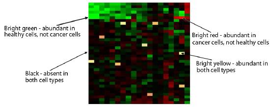
Figure 8.28 - Microarray analysis comparing gene expression in normal and cancer cells. Wikipedia
Unhybridized cDNAs are washed away and then the plate is analyzed. Red grid boxes correspond to an mRNA present in the cancerous tissue, but not in the non-cancerous tissue. Green grid boxes correspond to an mRNA present in the non-cancerous tissue, but not in the cancerous tissue. Yellow would correspond to mRNAs present in equal abundance in the two tissues (Figure 8.28). The intensity of each spot also gives information about the relative amounts of each mRNA in each tissue.

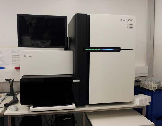
Figure 8.29 - Automated high throughput sequencer. Wikipedia
The same principle used for nucleic acid microarrays can be adapted for analyzing other molecules. For example, polypeptides could be bonded to the glass slide instead of DNA to create a protein chip. Protein chips are useful for studying the interactions of proteins with other molecules as well as for diagnostics.
RNA-Seq Technique
Like microarrays, a newer method called RNA-Seq, is a tool for simultaneously detecting and quantitating all of the transcripts in a given sample. This method relies on recently developed sequencing technologies called next-generation sequencing, or deep sequencing. These techniques allow for rapid, parallel sequencing of millions of DNA fragments and can, thus, be used not only for genomic DNA, but also to sequence all of the reverse-transcribed RNAs from a given sample.
To determine all the protein-coding genes that were being expressed in a particular set of cells under specific physiological conditions, all of the mRNA would first be extracted and reverse-transcribed into cDNA. This step is similar to the preparation of samples for microarrays. However, at this point, the cDNAs are fragmented into smaller pieces, and have small sequencing adapters attached at either end. The fragments are then subjected to high-throughput sequencing, to obtain short sequences from all of the fragments. These data are aligned against the genome sequence and used to measure the level of expression of different genes. RNA-Seq offers some advantages over microarrays. With microarrays, an RNA can only be detected if the gene sequence corresponding to it is present on the grid. In RNA-Seq every RNA present in the sample is sequenced, so detection of RNAs is not limited by the probes on a chip. RNA-Seq is more sensitive than microarrays and offers a much larger range over which gene expression can be measured accurately.

