3.4: Quantum Numbers
- Page ID
- 221387
\( \newcommand{\vecs}[1]{\overset { \scriptstyle \rightharpoonup} {\mathbf{#1}} } \)
\( \newcommand{\vecd}[1]{\overset{-\!-\!\rightharpoonup}{\vphantom{a}\smash {#1}}} \)
\( \newcommand{\id}{\mathrm{id}}\) \( \newcommand{\Span}{\mathrm{span}}\)
( \newcommand{\kernel}{\mathrm{null}\,}\) \( \newcommand{\range}{\mathrm{range}\,}\)
\( \newcommand{\RealPart}{\mathrm{Re}}\) \( \newcommand{\ImaginaryPart}{\mathrm{Im}}\)
\( \newcommand{\Argument}{\mathrm{Arg}}\) \( \newcommand{\norm}[1]{\| #1 \|}\)
\( \newcommand{\inner}[2]{\langle #1, #2 \rangle}\)
\( \newcommand{\Span}{\mathrm{span}}\)
\( \newcommand{\id}{\mathrm{id}}\)
\( \newcommand{\Span}{\mathrm{span}}\)
\( \newcommand{\kernel}{\mathrm{null}\,}\)
\( \newcommand{\range}{\mathrm{range}\,}\)
\( \newcommand{\RealPart}{\mathrm{Re}}\)
\( \newcommand{\ImaginaryPart}{\mathrm{Im}}\)
\( \newcommand{\Argument}{\mathrm{Arg}}\)
\( \newcommand{\norm}[1]{\| #1 \|}\)
\( \newcommand{\inner}[2]{\langle #1, #2 \rangle}\)
\( \newcommand{\Span}{\mathrm{span}}\) \( \newcommand{\AA}{\unicode[.8,0]{x212B}}\)
\( \newcommand{\vectorA}[1]{\vec{#1}} % arrow\)
\( \newcommand{\vectorAt}[1]{\vec{\text{#1}}} % arrow\)
\( \newcommand{\vectorB}[1]{\overset { \scriptstyle \rightharpoonup} {\mathbf{#1}} } \)
\( \newcommand{\vectorC}[1]{\textbf{#1}} \)
\( \newcommand{\vectorD}[1]{\overrightarrow{#1}} \)
\( \newcommand{\vectorDt}[1]{\overrightarrow{\text{#1}}} \)
\( \newcommand{\vectE}[1]{\overset{-\!-\!\rightharpoonup}{\vphantom{a}\smash{\mathbf {#1}}}} \)
\( \newcommand{\vecs}[1]{\overset { \scriptstyle \rightharpoonup} {\mathbf{#1}} } \)
\( \newcommand{\vecd}[1]{\overset{-\!-\!\rightharpoonup}{\vphantom{a}\smash {#1}}} \)
\(\newcommand{\avec}{\mathbf a}\) \(\newcommand{\bvec}{\mathbf b}\) \(\newcommand{\cvec}{\mathbf c}\) \(\newcommand{\dvec}{\mathbf d}\) \(\newcommand{\dtil}{\widetilde{\mathbf d}}\) \(\newcommand{\evec}{\mathbf e}\) \(\newcommand{\fvec}{\mathbf f}\) \(\newcommand{\nvec}{\mathbf n}\) \(\newcommand{\pvec}{\mathbf p}\) \(\newcommand{\qvec}{\mathbf q}\) \(\newcommand{\svec}{\mathbf s}\) \(\newcommand{\tvec}{\mathbf t}\) \(\newcommand{\uvec}{\mathbf u}\) \(\newcommand{\vvec}{\mathbf v}\) \(\newcommand{\wvec}{\mathbf w}\) \(\newcommand{\xvec}{\mathbf x}\) \(\newcommand{\yvec}{\mathbf y}\) \(\newcommand{\zvec}{\mathbf z}\) \(\newcommand{\rvec}{\mathbf r}\) \(\newcommand{\mvec}{\mathbf m}\) \(\newcommand{\zerovec}{\mathbf 0}\) \(\newcommand{\onevec}{\mathbf 1}\) \(\newcommand{\real}{\mathbb R}\) \(\newcommand{\twovec}[2]{\left[\begin{array}{r}#1 \\ #2 \end{array}\right]}\) \(\newcommand{\ctwovec}[2]{\left[\begin{array}{c}#1 \\ #2 \end{array}\right]}\) \(\newcommand{\threevec}[3]{\left[\begin{array}{r}#1 \\ #2 \\ #3 \end{array}\right]}\) \(\newcommand{\cthreevec}[3]{\left[\begin{array}{c}#1 \\ #2 \\ #3 \end{array}\right]}\) \(\newcommand{\fourvec}[4]{\left[\begin{array}{r}#1 \\ #2 \\ #3 \\ #4 \end{array}\right]}\) \(\newcommand{\cfourvec}[4]{\left[\begin{array}{c}#1 \\ #2 \\ #3 \\ #4 \end{array}\right]}\) \(\newcommand{\fivevec}[5]{\left[\begin{array}{r}#1 \\ #2 \\ #3 \\ #4 \\ #5 \\ \end{array}\right]}\) \(\newcommand{\cfivevec}[5]{\left[\begin{array}{c}#1 \\ #2 \\ #3 \\ #4 \\ #5 \\ \end{array}\right]}\) \(\newcommand{\mattwo}[4]{\left[\begin{array}{rr}#1 \amp #2 \\ #3 \amp #4 \\ \end{array}\right]}\) \(\newcommand{\laspan}[1]{\text{Span}\{#1\}}\) \(\newcommand{\bcal}{\cal B}\) \(\newcommand{\ccal}{\cal C}\) \(\newcommand{\scal}{\cal S}\) \(\newcommand{\wcal}{\cal W}\) \(\newcommand{\ecal}{\cal E}\) \(\newcommand{\coords}[2]{\left\{#1\right\}_{#2}}\) \(\newcommand{\gray}[1]{\color{gray}{#1}}\) \(\newcommand{\lgray}[1]{\color{lightgray}{#1}}\) \(\newcommand{\rank}{\operatorname{rank}}\) \(\newcommand{\row}{\text{Row}}\) \(\newcommand{\col}{\text{Col}}\) \(\renewcommand{\row}{\text{Row}}\) \(\newcommand{\nul}{\text{Nul}}\) \(\newcommand{\var}{\text{Var}}\) \(\newcommand{\corr}{\text{corr}}\) \(\newcommand{\len}[1]{\left|#1\right|}\) \(\newcommand{\bbar}{\overline{\bvec}}\) \(\newcommand{\bhat}{\widehat{\bvec}}\) \(\newcommand{\bperp}{\bvec^\perp}\) \(\newcommand{\xhat}{\widehat{\xvec}}\) \(\newcommand{\vhat}{\widehat{\vvec}}\) \(\newcommand{\uhat}{\widehat{\uvec}}\) \(\newcommand{\what}{\widehat{\wvec}}\) \(\newcommand{\Sighat}{\widehat{\Sigma}}\) \(\newcommand{\lt}{<}\) \(\newcommand{\gt}{>}\) \(\newcommand{\amp}{&}\) \(\definecolor{fillinmathshade}{gray}{0.9}\)If you attend a college or professional football game, you need a ticket to get in. It is very likely that your ticket may specify a gate number, section number, row, and seat number. No other ticket can have the same four parts to it. It may even have the same gate, section, and row, but it would still have to include a different seat number. Each seat is unique and allows only one occupant to fill it.
We use a series of specific numbers, called quantum numbers, to describe the location of an electron in an associated atom. Quantum numbers specify the properties of the atomic orbitals and the electrons in those orbitals. An electron in an atom or ion has four quantum numbers to describe its state. Think of them as important variables in an equation that describes the three-dimensional position of electrons in a given atom.
Principal Quantum Number \(\left( n \right)\)
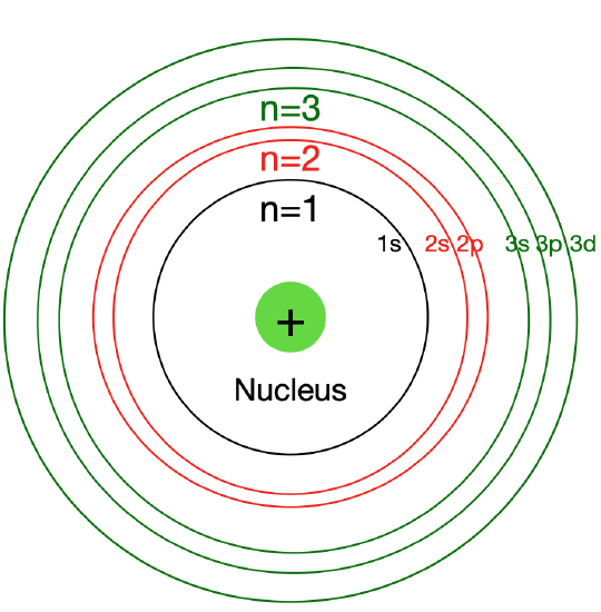
The principal quantum number, signified by \(n\), is the main energy level (shell) occupied by the electron. Energy levels are fixed distances from the nucleus of a given atom. They are described in whole number increments (e.g., 1, 2, 3, 4, 5, 6, ...). At location \(n=1\), an electron would be closest to the nucleus, while at \(n=2\) the electron would be farther, and at \(n=3\) farther yet. As we will see, the principal quantum number corresponds to the row number for an atom on the periodic table.

Figure \(\PageIndex{1}\): In Bohr´s atomic model, Principal Quantum Number \(\left( n \right)\) can be interpreted as the different "energy levels" around the nucleus.
Angular Momentum Quantum Number \(\left( l \right)\)
The angular momentum quantum number, signified by \(l\), describes the energy sublevel (subshell) and general shape or region an electron occupies—its orbital shape. The value of \(l\) depends on the value of the principal quantum number, \(n\). The angular momentum quantum number can have positive values of zero to \(\left( n-1 \right)\). If \(n=2\), \(l\) could be either \(0\) or \(1\).
Instead of using numbers to designate \(l=0\), we use letters:
If \(l=0\), then it’s called s
If or \(l=1\), then it’s called p
If \(l=2\) then it’s called d
If \(l=3\), then it’s called f
Each type of subshell (or letter) has a very specific shape, as described on the orbital shapes page.

Figure \(\PageIndex{2}\): In Bohr´s atomic model, Angular Momentum Quantum Number \(\left( l \right)\) can be interpreted as the different "energy sublevels" within each energy level
Magnetic Quantum Number \(\left( m_l \right)\)
The magnetic quantum number, signified as \(m_l\), describes a particular orbital (box) and the orbital orientation in space. Electrons can be situated in one of three planes in three dimensional space around a given nucleus (\(x\), \(y\), and \(z\)). For a given value of the angular momentum quantum number, \(l\), there can be \(\left( 2l+1 \right)\) values for \(m_l\). As an example:
\(n=2\)
\(l=0\) or \(1\)
for \(l=0\), \(m_l = 0\)
for \(l=1\), \(m_l = -1, 0, +1\)
| Principal Energy Level | Number of Possible Sublevels | Possible Angular Momentum Quantum Numbers | Orbital Designation by Principal Energy Level and Sublevel |
|---|---|---|---|
| \(n=1\) | 1 | \(l=0\) or \(l=s\) | \(1s\) |
| \(n=2\) | 2 | \(l=0\) or \(l=s\) | \(2s\) |
| \(l=1\) or \(l=p\) | \(2p\) | ||
| \(n=3\) | 3 | \(l=0\) or \(l=s\) | \(3s\) |
| \(l=1\) or \(l=p\) | \(3p\) | ||
| \(l=2\) or \(l=d\) | \(3d\) | ||
| \(n=4\) | 4 | \(l=0\) or \(l=s\) | \(4s\) |
| \(l=1\) or \(l=p\) | \(4p\) | ||
| \(l=2\) or \(l=d\) | \(4d\) | ||
| \(l=3\) or \(l=f\) | \(4f\) |
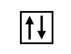
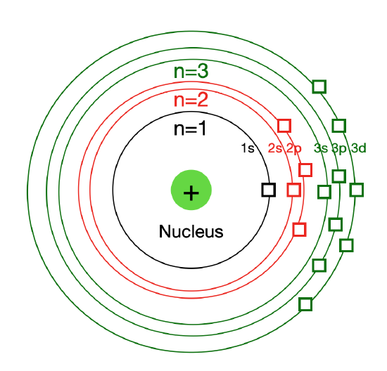
The table above shows the possible angular momentum quantum number values \(\left( l \right)\) for the corresponding principal quantum numbers \(\left( n \right) of \(n = 1, n=2, n=3,\) and \(n=4\). A single orbital can hold a maximum of two electrons, and it can represented as a single box. Although each one of this boxes has a specific shape given by its \(m_l\) number (check next section)

The total number of orbital per energy sublevel can be represented as:

Figure \(\PageIndex{3}\): In Bohr´s atomic model, Magnetic Quantum Number \(\left( m_l \right)\) can be considered as a "box" or a seat within each energy subshell. The number of "seats" depends on the type of subshell (s, p, d, or f).
Spin Quantum Number \(\left( m_s \right)\)
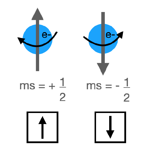
The spin quantum number describes the spin for a given electron. An electron can have one of two associated spins, \(\left( + \frac{1}{2} \right)\) spin, or \(\left( -\frac{1}{2} \right)\) spin. An electron cannot have zero spin. We also represent spin with arrows \(\uparrow\) or \(\downarrow\). A single orbital can hold a maximum of two electrons, and each must have opposite spin.
The electron spin describes the “rotation” or “spinning” of each electron around its own axis. Each electron acts as a tiny magnet that can rotate to the left \(\left( + \frac{1}{2} \right)\) or to the right or \(\left( -\frac{1}{2} \right)\).

Figure \(\PageIndex{1}\): In Bohr´s atomic model, Spin Quantum Number \(\left( m_s \right)\) can be interpreted a sthwo possible direction in which the electron can rotate around its axis.
Summary
- Quantum numbers specify the arrangements of electrons in orbitals.
- There are four quantum numbers that provide information about various aspects of electron behavior.

