9.3: The Overlap Integral
- Page ID
- 204573
\( \newcommand{\vecs}[1]{\overset { \scriptstyle \rightharpoonup} {\mathbf{#1}} } \)
\( \newcommand{\vecd}[1]{\overset{-\!-\!\rightharpoonup}{\vphantom{a}\smash {#1}}} \)
\( \newcommand{\id}{\mathrm{id}}\) \( \newcommand{\Span}{\mathrm{span}}\)
( \newcommand{\kernel}{\mathrm{null}\,}\) \( \newcommand{\range}{\mathrm{range}\,}\)
\( \newcommand{\RealPart}{\mathrm{Re}}\) \( \newcommand{\ImaginaryPart}{\mathrm{Im}}\)
\( \newcommand{\Argument}{\mathrm{Arg}}\) \( \newcommand{\norm}[1]{\| #1 \|}\)
\( \newcommand{\inner}[2]{\langle #1, #2 \rangle}\)
\( \newcommand{\Span}{\mathrm{span}}\)
\( \newcommand{\id}{\mathrm{id}}\)
\( \newcommand{\Span}{\mathrm{span}}\)
\( \newcommand{\kernel}{\mathrm{null}\,}\)
\( \newcommand{\range}{\mathrm{range}\,}\)
\( \newcommand{\RealPart}{\mathrm{Re}}\)
\( \newcommand{\ImaginaryPart}{\mathrm{Im}}\)
\( \newcommand{\Argument}{\mathrm{Arg}}\)
\( \newcommand{\norm}[1]{\| #1 \|}\)
\( \newcommand{\inner}[2]{\langle #1, #2 \rangle}\)
\( \newcommand{\Span}{\mathrm{span}}\) \( \newcommand{\AA}{\unicode[.8,0]{x212B}}\)
\( \newcommand{\vectorA}[1]{\vec{#1}} % arrow\)
\( \newcommand{\vectorAt}[1]{\vec{\text{#1}}} % arrow\)
\( \newcommand{\vectorB}[1]{\overset { \scriptstyle \rightharpoonup} {\mathbf{#1}} } \)
\( \newcommand{\vectorC}[1]{\textbf{#1}} \)
\( \newcommand{\vectorD}[1]{\overrightarrow{#1}} \)
\( \newcommand{\vectorDt}[1]{\overrightarrow{\text{#1}}} \)
\( \newcommand{\vectE}[1]{\overset{-\!-\!\rightharpoonup}{\vphantom{a}\smash{\mathbf {#1}}}} \)
\( \newcommand{\vecs}[1]{\overset { \scriptstyle \rightharpoonup} {\mathbf{#1}} } \)
\( \newcommand{\vecd}[1]{\overset{-\!-\!\rightharpoonup}{\vphantom{a}\smash {#1}}} \)
\(\newcommand{\avec}{\mathbf a}\) \(\newcommand{\bvec}{\mathbf b}\) \(\newcommand{\cvec}{\mathbf c}\) \(\newcommand{\dvec}{\mathbf d}\) \(\newcommand{\dtil}{\widetilde{\mathbf d}}\) \(\newcommand{\evec}{\mathbf e}\) \(\newcommand{\fvec}{\mathbf f}\) \(\newcommand{\nvec}{\mathbf n}\) \(\newcommand{\pvec}{\mathbf p}\) \(\newcommand{\qvec}{\mathbf q}\) \(\newcommand{\svec}{\mathbf s}\) \(\newcommand{\tvec}{\mathbf t}\) \(\newcommand{\uvec}{\mathbf u}\) \(\newcommand{\vvec}{\mathbf v}\) \(\newcommand{\wvec}{\mathbf w}\) \(\newcommand{\xvec}{\mathbf x}\) \(\newcommand{\yvec}{\mathbf y}\) \(\newcommand{\zvec}{\mathbf z}\) \(\newcommand{\rvec}{\mathbf r}\) \(\newcommand{\mvec}{\mathbf m}\) \(\newcommand{\zerovec}{\mathbf 0}\) \(\newcommand{\onevec}{\mathbf 1}\) \(\newcommand{\real}{\mathbb R}\) \(\newcommand{\twovec}[2]{\left[\begin{array}{r}#1 \\ #2 \end{array}\right]}\) \(\newcommand{\ctwovec}[2]{\left[\begin{array}{c}#1 \\ #2 \end{array}\right]}\) \(\newcommand{\threevec}[3]{\left[\begin{array}{r}#1 \\ #2 \\ #3 \end{array}\right]}\) \(\newcommand{\cthreevec}[3]{\left[\begin{array}{c}#1 \\ #2 \\ #3 \end{array}\right]}\) \(\newcommand{\fourvec}[4]{\left[\begin{array}{r}#1 \\ #2 \\ #3 \\ #4 \end{array}\right]}\) \(\newcommand{\cfourvec}[4]{\left[\begin{array}{c}#1 \\ #2 \\ #3 \\ #4 \end{array}\right]}\) \(\newcommand{\fivevec}[5]{\left[\begin{array}{r}#1 \\ #2 \\ #3 \\ #4 \\ #5 \\ \end{array}\right]}\) \(\newcommand{\cfivevec}[5]{\left[\begin{array}{c}#1 \\ #2 \\ #3 \\ #4 \\ #5 \\ \end{array}\right]}\) \(\newcommand{\mattwo}[4]{\left[\begin{array}{rr}#1 \amp #2 \\ #3 \amp #4 \\ \end{array}\right]}\) \(\newcommand{\laspan}[1]{\text{Span}\{#1\}}\) \(\newcommand{\bcal}{\cal B}\) \(\newcommand{\ccal}{\cal C}\) \(\newcommand{\scal}{\cal S}\) \(\newcommand{\wcal}{\cal W}\) \(\newcommand{\ecal}{\cal E}\) \(\newcommand{\coords}[2]{\left\{#1\right\}_{#2}}\) \(\newcommand{\gray}[1]{\color{gray}{#1}}\) \(\newcommand{\lgray}[1]{\color{lightgray}{#1}}\) \(\newcommand{\rank}{\operatorname{rank}}\) \(\newcommand{\row}{\text{Row}}\) \(\newcommand{\col}{\text{Col}}\) \(\renewcommand{\row}{\text{Row}}\) \(\newcommand{\nul}{\text{Nul}}\) \(\newcommand{\var}{\text{Var}}\) \(\newcommand{\corr}{\text{corr}}\) \(\newcommand{\len}[1]{\left|#1\right|}\) \(\newcommand{\bbar}{\overline{\bvec}}\) \(\newcommand{\bhat}{\widehat{\bvec}}\) \(\newcommand{\bperp}{\bvec^\perp}\) \(\newcommand{\xhat}{\widehat{\xvec}}\) \(\newcommand{\vhat}{\widehat{\vvec}}\) \(\newcommand{\uhat}{\widehat{\uvec}}\) \(\newcommand{\what}{\widehat{\wvec}}\) \(\newcommand{\Sighat}{\widehat{\Sigma}}\) \(\newcommand{\lt}{<}\) \(\newcommand{\gt}{>}\) \(\newcommand{\amp}{&}\) \(\definecolor{fillinmathshade}{gray}{0.9}\)For \(\ce{H2^{+}}\), the simplest molecule, we must determine the values for the coefficients, \(C_A\) and \(C_B\) for the LCAO approximation for the molecular orbital as a linear combination of the two atomic orbitals
\[ |\psi (r) \rangle = C_A 1s_A (r) + C_B1s_B (r) \]
We could use the linear variational method to find a value for these coefficients, but for the case of \(\ce{H2^{+}}\) evaluating these coefficients is easy. Since the two protons are identical, the probability that the electron is near \(A\) must equal the probability that the electron is near \(B\). These probabilities are given by \(|C_A|^2\) and \(|C_B|^2\), respectively. Consider two possibilities that satisfy the condition
\[|C_A|^2 = |C_B|^2\]
so \(C_A = C_B = C_{+}\) and \(C_A = -C_B = C_{-}\). These two cases produce two molecular orbitals:
\[\underbrace{| \psi _+ \rangle = C_+(1s_A + 1s_B)}_{\text{bonding molecular orbital}} \label{9.3.1a}\]
and
\[\underbrace{| \psi _{-} \rangle = C_{-}(1s_A - 1s_B)}_{\text{antibonding molecular orbital}} \label{9.3.1b}\]
The probability density for finding the electron at any point in space is given by \(|{\psi}^2|\) and the electronic charge density is just \(|e{\psi}^2|\). The important difference between \(\psi _+\) and \(\psi _{-}\) is that the charge density for \(| \psi_+ \rangle\) is enhanced between the two protons, whereas it is diminished for \(|\psi _{-} \rangle\) as shown in Figures \(\PageIndex{1}\). \(\psi _{-}\) has a node in the middle while \(| \psi_+ \rangle\) corresponds to our intuitive sense of what a chemical bond must be like. The electronic charge density is enhanced in the region between the two protons. So \(|\psi_+ \rangle\) is called a bonding molecular orbital. If the electron were described by \(|\psi _{-} \rangle\), the low charge density between the two protons would not balance the Coulomb repulsion of the protons, so \(|\psi _{-} \rangle\) is called an antibonding molecular orbital.
Now we want to evaluate \(C_+\) and \(C_-\) and then calculate the energy. The bonding and antibonding character of \(\psi _+\) and \(\psi _{-}\) also should be reflected in the energy. If \( |\psi _+ \rangle\) indeed describes a bonding orbital, then the energy of this state should be less than that of a proton and hydrogen atom that are separated. The calculation of the energy will tell us whether this simple theory predicts H2+ to be stable or not and also how much energy is required to dissociate this molecule.
The constants \(C_+\) and \(C_-\) are evaluated from the standard normalization condition:
\[ \begin{align} \int \psi ^*_{\pm} \psi _{\pm} d\tau = \left \langle \psi _{\pm} | \psi _{\pm} \right \rangle &= 1 \label {9.3.1} \\[4pt] \left \langle C_{\pm} ( 1s_A \pm 1s_B ) | C_{\pm} ( 1s_A \pm 1s_B ) \right \rangle &= 1 \label {9.3.2} \\[4pt] |C_\pm|^2 [ \underbrace{\langle1s_A | 1s_A \rangle }_{1} + \underbrace{\langle 1s_B | 1s_B \rangle}_{1} \pm \underbrace{ \langle1s_B | 1s_A\rangle}_{S} \pm \underbrace{ \langle1s_A | 1s_B \rangle}_{S^*}] &= 1 \label {9.3.3} \end{align} \]
Since the atomic orbitals are normalized, the first two integrals are just 1. The last two integrals are called overlap integrals and are symbolized by \(S\) and \(S^*\), respectively, since one is the complex conjugate of the other.
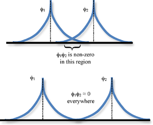
The overlap integrals are telling us to take the value of 1sB at a point multiply by the value of 1sA at that point and sum (integrate) such a product over all of space (Figure \(\PageIndex{1}\)). If the functions do not overlap, i.e. if one is zero when the other one is not and vice versa, these integrals then will be zero. It also is possible in general for such integrals to be zero even if the functions overlap because of the cancelation of positive and negative contributions.

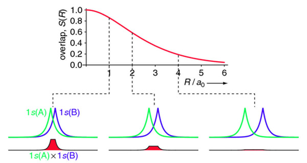
If the overlap integral is zero, for whatever reason, the functions are said to be orthogonal. Notice that the overlap integral ranges from 0 to 1 as the separation between the protons varies from \(R = ∞\) to \(R = 0\). Clearly when the protons are infinite distance apart, there is no overlap, and when \(R = 0\) both functions are centered on one nucleus and \(\left \langle 1s_A | 1s_B \right \rangle\) becomes identical to \(\left \langle 1s_B | 1s_A \right \rangle\), which is normalized to 1, because \(1s_A = 1s_B\).
With these considerations and using the fact that \(1s\) wavefunctions are real so
\[ \left \langle 1s_A | 1s_B \right \rangle = \left \langle 1s_B | 1s_A \right \rangle = S \label {9.3.4}\]
Equation \(\ref{9.3.3}\) becomes
\[|C_{\pm}|^2 (2 \pm 2S ) = 1 \label {9.3.5}\]
The solution to Equation \(\ref{9.3.5}\) is given by
\[ C_{\pm} = \dfrac{1}{\sqrt{2(1 \pm S )}} \label {9.3.6}\]
Hence, the normalized molecular orbitals in Equations \(\ref{9.3.1a}\) and \(\ref{9.3.1a}\) are
\[| \psi _+\rangle = \dfrac{1}{\sqrt{2(1 + S )}} (1s_A + 1s_B) \label{9.3.7a}\]
and
\[|\psi _{-} \rangle = \dfrac{1}{\sqrt{2(1 - S )}} (1s_A - 1s_B) \label{9.3.7b}\]
The energies associated with these wavefunctions requires a bit more effort to calculate though as demonstrated in the following section.
For the overlap integral of two 1s orbitals from the hydrogen dimer discussed above is difficult to evaluate analytically and is explained here. The final answer is:
\[ \begin{align} S(R) &= \left \langle 1s_A | 1s_B \right \rangle \\[4pt] &= e^{-R/a_o} \left( 1 +\dfrac{R}{a_o} + \dfrac{R^2}{3a_o^2} \right) \label{overlap} \end{align}\]
The overlap integral for two 1s atomic orbitals of hydrogen is graphically displayed below

Example \(\PageIndex{1}\)
Calculate the difference in the electronic charge density (C/pm3) at a point halfway between the two nuclei for \(\ce{H2^{+}}\) for an electron in the bonding molecular orbital compared to one in the antibonding molecular orbital.
Solution
The electronic charge density is calculated with the formula \(|e{\psi}^2|\) where \(e = 1.602 \times 10^{-19} C\)
a: Bonding Molecular Orbital
First, squaring the bonding molecular orbital (Equation \ref{9.3.7a}) gives us:
\[ \begin{align*} \psi_+^2 &=\dfrac{1}{2(1 + S )} (1s_A+1s_B)^2 \\[4pt] &= \dfrac{1}{2(1 + S )} \dfrac{1}{\pi a_0^3}\Big(e^{-r_A/a_0}+e^{-r_B/a_0}\Big)^2 \\[4pt] &= \dfrac{1}{2(1 + S )} \dfrac{1}{\pi a_0^3} \\[4pt] &= (0.561)^2\times\left(\dfrac{1}{\pi\times(52.9\;\text{pm})^3}\right)=6.7672\times10^{-7}\;\text{pm}^{-3} \end{align*}\]
(Note: The value of \(C^2\) is obtained from equation 9.3.12 and the value of S is from Equation \ref{overlap})
To find the density at halfway between A and B for the bonding orbital evalulate at 1/2 R,
\(r_A=\dfrac{1}{2}R\) and \(r_B=\dfrac{1}{2}R\)
\[\psi_+^2=3.7\times10^{-7}\;\text{pm}^{-3}\]
Now multiply this answer by e to generate the electronic charge density,
\[P = \Big(3.7\times10^{-7}\;\text{pm}^{-3}\Big)\times\Big(1.602\times10^{-19}\Big)\;\text{C} = 5.93\times10^{-26} C/pm^{3}\]
b: Antibonding Molecular Orbital
To find the halfway between A and B for the anti-bonding orbital at \(r_A=\dfrac{1}{2}R\) and \(r_B=\dfrac{1}{2}R\). However, simple inspection of Equation \ref{9.3.7b} or Figure \(\PageIndex{1}\) shows this will be zero.
\[\text{e}\psi_-^2=0\]
Obviously, when multiplied by e, the answer is still zero. This makes logical sense as there would be no charge density between the two atoms as there lies a node with no probability of finding an electron.
Exercise \(\PageIndex{1}\)
Show that for two arbitrary functions \(\left \langle \varphi _B | \varphi _A \right \rangle \) is the complex conjugate of \(\left \langle \varphi _A | \varphi _B \right \rangle \) and that these two integrals are equal if the functions are real.
Contributors
David M. Hanson, Erica Harvey, Robert Sweeney, Theresa Julia Zielinski ("Quantum States of Atoms and Molecules")

