
8.6: Antisymmetric Wavefunctions can be Represented by Slater Determinants
- Page ID
- 204563
\( \newcommand{\vecs}[1]{\overset { \scriptstyle \rightharpoonup} {\mathbf{#1}} } \)
\( \newcommand{\vecd}[1]{\overset{-\!-\!\rightharpoonup}{\vphantom{a}\smash {#1}}} \)
\( \newcommand{\id}{\mathrm{id}}\) \( \newcommand{\Span}{\mathrm{span}}\)
( \newcommand{\kernel}{\mathrm{null}\,}\) \( \newcommand{\range}{\mathrm{range}\,}\)
\( \newcommand{\RealPart}{\mathrm{Re}}\) \( \newcommand{\ImaginaryPart}{\mathrm{Im}}\)
\( \newcommand{\Argument}{\mathrm{Arg}}\) \( \newcommand{\norm}[1]{\| #1 \|}\)
\( \newcommand{\inner}[2]{\langle #1, #2 \rangle}\)
\( \newcommand{\Span}{\mathrm{span}}\)
\( \newcommand{\id}{\mathrm{id}}\)
\( \newcommand{\Span}{\mathrm{span}}\)
\( \newcommand{\kernel}{\mathrm{null}\,}\)
\( \newcommand{\range}{\mathrm{range}\,}\)
\( \newcommand{\RealPart}{\mathrm{Re}}\)
\( \newcommand{\ImaginaryPart}{\mathrm{Im}}\)
\( \newcommand{\Argument}{\mathrm{Arg}}\)
\( \newcommand{\norm}[1]{\| #1 \|}\)
\( \newcommand{\inner}[2]{\langle #1, #2 \rangle}\)
\( \newcommand{\Span}{\mathrm{span}}\) \( \newcommand{\AA}{\unicode[.8,0]{x212B}}\)
\( \newcommand{\vectorA}[1]{\vec{#1}} % arrow\)
\( \newcommand{\vectorAt}[1]{\vec{\text{#1}}} % arrow\)
\( \newcommand{\vectorB}[1]{\overset { \scriptstyle \rightharpoonup} {\mathbf{#1}} } \)
\( \newcommand{\vectorC}[1]{\textbf{#1}} \)
\( \newcommand{\vectorD}[1]{\overrightarrow{#1}} \)
\( \newcommand{\vectorDt}[1]{\overrightarrow{\text{#1}}} \)
\( \newcommand{\vectE}[1]{\overset{-\!-\!\rightharpoonup}{\vphantom{a}\smash{\mathbf {#1}}}} \)
\( \newcommand{\vecs}[1]{\overset { \scriptstyle \rightharpoonup} {\mathbf{#1}} } \)
\( \newcommand{\vecd}[1]{\overset{-\!-\!\rightharpoonup}{\vphantom{a}\smash {#1}}} \)
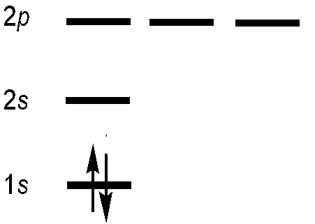
\(\newcommand{\avec}{\mathbf a}\) \(\newcommand{\bvec}{\mathbf b}\) \(\newcommand{\cvec}{\mathbf c}\) \(\newcommand{\dvec}{\mathbf d}\) \(\newcommand{\dtil}{\widetilde{\mathbf d}}\) \(\newcommand{\evec}{\mathbf e}\) \(\newcommand{\fvec}{\mathbf f}\) \(\newcommand{\nvec}{\mathbf n}\) \(\newcommand{\pvec}{\mathbf p}\) \(\newcommand{\qvec}{\mathbf q}\) \(\newcommand{\svec}{\mathbf s}\) \(\newcommand{\tvec}{\mathbf t}\) \(\newcommand{\uvec}{\mathbf u}\) \(\newcommand{\vvec}{\mathbf v}\) \(\newcommand{\wvec}{\mathbf w}\) \(\newcommand{\xvec}{\mathbf x}\) \(\newcommand{\yvec}{\mathbf y}\) \(\newcommand{\zvec}{\mathbf z}\) \(\newcommand{\rvec}{\mathbf r}\) \(\newcommand{\mvec}{\mathbf m}\) \(\newcommand{\zerovec}{\mathbf 0}\) \(\newcommand{\onevec}{\mathbf 1}\) \(\newcommand{\real}{\mathbb R}\) \(\newcommand{\twovec}[2]{\left[\begin{array}{r}#1 \\ #2 \end{array}\right]}\) \(\newcommand{\ctwovec}[2]{\left[\begin{array}{c}#1 \\ #2 \end{array}\right]}\) \(\newcommand{\threevec}[3]{\left[\begin{array}{r}#1 \\ #2 \\ #3 \end{array}\right]}\) \(\newcommand{\cthreevec}[3]{\left[\begin{array}{c}#1 \\ #2 \\ #3 \end{array}\right]}\) \(\newcommand{\fourvec}[4]{\left[\begin{array}{r}#1 \\ #2 \\ #3 \\ #4 \end{array}\right]}\) \(\newcommand{\cfourvec}[4]{\left[\begin{array}{c}#1 \\ #2 \\ #3 \\ #4 \end{array}\right]}\) \(\newcommand{\fivevec}[5]{\left[\begin{array}{r}#1 \\ #2 \\ #3 \\ #4 \\ #5 \\ \end{array}\right]}\) \(\newcommand{\cfivevec}[5]{\left[\begin{array}{c}#1 \\ #2 \\ #3 \\ #4 \\ #5 \\ \end{array}\right]}\) \(\newcommand{\mattwo}[4]{\left[\begin{array}{rr}#1 \amp #2 \\ #3 \amp #4 \\ \end{array}\right]}\) \(\newcommand{\laspan}[1]{\text{Span}\{#1\}}\) \(\newcommand{\bcal}{\cal B}\) \(\newcommand{\ccal}{\cal C}\) \(\newcommand{\scal}{\cal S}\) \(\newcommand{\wcal}{\cal W}\) \(\newcommand{\ecal}{\cal E}\) \(\newcommand{\coords}[2]{\left\{#1\right\}_{#2}}\) \(\newcommand{\gray}[1]{\color{gray}{#1}}\) \(\newcommand{\lgray}[1]{\color{lightgray}{#1}}\) \(\newcommand{\rank}{\operatorname{rank}}\) \(\newcommand{\row}{\text{Row}}\) \(\newcommand{\col}{\text{Col}}\) \(\renewcommand{\row}{\text{Row}}\) \(\newcommand{\nul}{\text{Nul}}\) \(\newcommand{\var}{\text{Var}}\) \(\newcommand{\corr}{\text{corr}}\) \(\newcommand{\len}[1]{\left|#1\right|}\) \(\newcommand{\bbar}{\overline{\bvec}}\) \(\newcommand{\bhat}{\widehat{\bvec}}\) \(\newcommand{\bperp}{\bvec^\perp}\) \(\newcommand{\xhat}{\widehat{\xvec}}\) \(\newcommand{\vhat}{\widehat{\vvec}}\) \(\newcommand{\uhat}{\widehat{\uvec}}\) \(\newcommand{\what}{\widehat{\wvec}}\) \(\newcommand{\Sighat}{\widehat{\Sigma}}\) \(\newcommand{\lt}{<}\) \(\newcommand{\gt}{>}\) \(\newcommand{\amp}{&}\) \(\definecolor{fillinmathshade}{gray}{0.9}\)Let’s try to construct an antisymmetric function that describes the two electrons in the ground state of helium. Blindly following the first statement of the Pauli Exclusion Principle, then each electron in a multi-electron atom must be described by a different spin-orbital. For the ground-state helium atom, this gives a \(1s^22s^02p^0\) configuration (Figure \(\PageIndex{1}\)).
We try constructing a simple product wavefunction for helium using two different spin-orbitals. Both have the 1s spatial component, but one has spin function \(\alpha\) and the other has spin function \(\beta\) so the product wavefunction matches the form of the ground state electron configuration for He, \(1s^2\).
\[ | \psi (\mathbf{r}_1, \mathbf{r}_2 ) \rangle = \varphi _{1s\alpha} (\mathbf{r}_1) \varphi _{1s\beta} ( \mathbf{r}_2) \label {8.6.1}\]
After permutation of the electrons, this becomes
\[ | \psi ( \mathbf{r}_2,\mathbf{r}_1 ) \rangle = \varphi _{1s\alpha} ( \mathbf{r}_2) \varphi _{1s\beta} (\mathbf{r}_1) \label {8.6.2}\]
which is different from the starting function since \(\varphi _{1s\alpha}\) and \(\varphi _{1s\beta}\) are different spin-orbital functions. Hence, the simple product wavefunction in Equation \ref{8.6.1} does not satisfy the indistinguishability requirement since an antisymmetric function must produce the same function multiplied by (–1) after permutation of two electrons, and that is not the case here. We must try something else. To avoid getting a totally different function when we permute the electrons, we can make a linear combination of functions. A very simple way of taking a linear combination involves making a new function by simply adding or subtracting functions. The function that is created by subtracting the right-hand side of Equation \(\ref{8.6.2}\) from the right-hand side of Equation \(\ref{8.6.1}\) has the desired antisymmetric behavior. The constant on the right-hand side accounts for the fact that the total wavefunction must be normalized.
\[ | \psi (\mathbf{r}_1, \mathbf{r}_2) \rangle = \dfrac {1}{\sqrt {2}} [ \varphi _{1s\alpha}(\mathbf{r}_1) \varphi _{1s\beta}( \mathbf{r}_2) - \varphi _{1s\alpha}( \mathbf{r}_2) \varphi _{1s\beta}(\mathbf{r}_1)] \label{8.6.3} \] We can introduce a shorthand notation for the arbitrary spin-orbital
\[ \varphi_{i\alpha}(\mathbf{r_j}) = \varphi_i \alpha(j)\]
or
\[ \varphi_{i\beta}(\mathbf{r_j}) = \varphi_i \beta(j)\]
as determined by the \(m_s\) quantum number. This wavefunction in Equation \ref{8.6.3} can be decomposed into spatial and spin components:
\[ | \psi (\mathbf{r}_1, \mathbf{r}_2) \rangle = \dfrac {1}{\sqrt {2}} \underbrace{[ \varphi _{1s}(1) \varphi _{1s}(2)]}_{\text{spatial component}} \underbrace{[ \alpha(1) \beta( 2) - \alpha( 2) \beta(1)]}_{\text{spin component}} \label{8.6.3B} \]
Exercise \(\PageIndex{1}\)
Show that the linear combination in Equation \(\ref{8.6.3}\) is antisymmetric with respect to permutation of the two electrons. (Hint: replace the minus sign with a plus sign (i.e. take the positive linear combination of the same two functions) and show that the resultant linear combination is symmetric).
- Answer
-
\(| \Psi(r 1, r 2)>=1 / \sqrt{2}[\varphi 1 s \alpha(r)) \varphi 1 s \beta(r 2)-\varphi 1 s \beta(r 2)-\varphi 1 s \alpha(r 2) \varphi 1 s \beta(r 1)](8.6 .3) \rightarrow\)show this is antisymmetric
Change the minus sign to plus sign show this is symmetric
(1) \(| \Psi(r 1, r 2)>=1 / \sqrt{2}[\varphi 1 s \alpha(r 1) \varphi 1 s \beta(r 2)-\varphi 1 s \alpha(r 2) \varphi 1 s \beta(r 1)]\)
(2) \(| \Psi(r 1, r 2)>=1 / \sqrt{2}[\varphi 1 \operatorname{sa}(r 1) \varphi 1 s \beta(r 2)+\varphi 1 s \alpha(r 2) \varphi 1 s \beta(r 1)]\)To see if symmetric \(\left|\Psi_{(r 1, r 2)}>=\right| \Psi(r 2, r 1)>\) \(| \Psi(r 1, r 2)>=1 / \sqrt{2}[\varphi 1 s a(r 1) \varphi 1 s \beta(r 2)+\varphi 1 s \alpha(r 2) \varphi 1 s \beta(r 1)]=\)
\(| \Psi(r 2, r 1)>=1 / \sqrt{2}[\varphi 1 s \alpha(r 2) \varphi 1 s \beta(r 1)+\varphi 1 s \alpha(r 1) \varphi 1 s \beta(r 2)]\)
Can rearrange and \(| \Psi(r 1, r 2)>=1 / \sqrt{2}[\varphi 1 s \alpha(r 1) \varphi 1 s \beta(r 2)+\varphi 1 s \alpha(r 2) \varphi 1 s \beta(r 1)]=\)
\(| \Psi(r 1, r 2)>=1 / \sqrt{2}[\varphi 1 s \alpha(r 1) \varphi 1 s \beta(r 2)+\varphi 1 s \alpha(r 2) \varphi 1 s \beta(r 1)]\)
So \(| \Psi(r 1, r 2)>=1 / \sqrt{2}[\varphi 1 \operatorname{sa}(r 1) \varphi 1 s \beta(r 2)+\varphi 1 s \alpha(r 2) \varphi 1 s \beta(r 1)]\) is symmetric
Now for antisymmetric \(|\Psi(r 1, r 2)>=-| \Psi(r 2, r 1)>\) \(| \Psi(r 1, r 2)>=1 / \sqrt{2}[\varphi 1 s \alpha(r 1) \varphi 1 s \beta(r 2)-\varphi 1 s \alpha(r 2) \varphi 1 s \beta(r 1)]=\)
\(| \Psi(r 2, r 1)>=-1 / \sqrt{2}[\varphi 1 s \alpha(r 2) \varphi 1 s \beta(r 1)-\varphi 1 s \alpha(r 1) \varphi 1 s \beta(r 2)]\)Simplify equation above and \(1 / \sqrt{2}[\varphi 1 s \alpha(r 1) \varphi 1 s \beta(r 2)-\varphi 1 s \alpha(r 2) \varphi 1 s \beta(r 1)]=1 / \sqrt{2}[\varphi 1 s \alpha(r 1) \varphi 1 s \beta(r 2)-\varphi 1 s \alpha(r 2) \varphi 1 s \beta(r 1)]\)
\[|\Psi(r 1, r 2)>\quad-| \Psi(r 2, r 1)>\]
\(\left|\Psi_{(r 1, r 2)}\right\rangle= 1 / \sqrt{2}[\varphi 1 s \alpha(r 1) \varphi 1 s \beta(r 2)-\varphi 1 s \alpha(r 2) \varphi 1 s \beta(r 1)] \rightarrow\) is antisymmetric
The first excited state of He is \(1s^12s^12p^0\) and we can envision four microstates for this configuration (Figure \(\PageIndex{2}\)) that also must satisfy indistinguishability requirement just like the ground state.
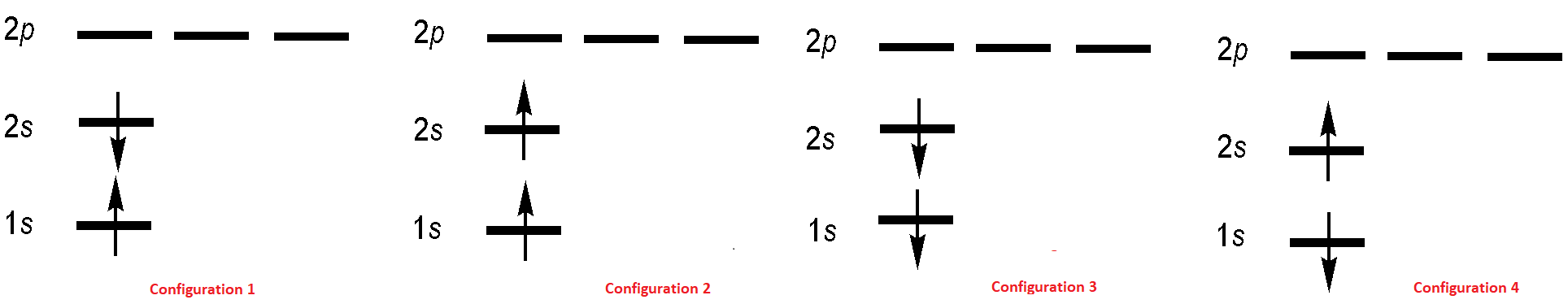
These electron configurations are used to construct four possible excited-state two-electron wavefunctions (but not necessarily in a one-to-on correspondence):
\[ \begin{align} | \psi_1 (\mathbf{r}_1, \mathbf{r}_2) \rangle &= \dfrac {1}2 \underbrace{[ \varphi _{1s}(1) \varphi _{2s}(2)+\varphi _{1s}(2) \varphi _{2s}(1)]}_{\text{spatial component}} \underbrace{[ \alpha(1) \beta( 2) - \alpha( 2) \beta(1)]}_{\text{spin component}} \label{8.6.3C1} \\[4pt] | \psi_2 (\mathbf{r}_1, \mathbf{r}_2) \rangle &= \dfrac {1}{\sqrt {2}} \underbrace{[ \varphi _{1s}(1) \varphi _{2s}(2) - \varphi _{1s}(2) \varphi _{2s}(1)]}_{\text{spatial component}} \underbrace{[ \alpha(1) \alpha( 2)]}_{\text{spin component}} \label{8.6.3C2} \\[4pt] | \psi_3 (\mathbf{r}_1, \mathbf{r}_2) \rangle &= \dfrac {1}{\sqrt {2}} \underbrace{[ \varphi _{1s}(1) \varphi _{2s}(2) - \varphi _{1s}(2) \varphi _{2s}(1)]}_{\text{spatial component}} \underbrace{[ \alpha(1) \beta( 2) + \alpha( 2) \beta(1)]}_{\text{spin component}} \label{8.6.3C3} \\[4pt] | \psi_4 (\mathbf{r}_1, \mathbf{r}_2) \rangle &= \dfrac {1}2 \underbrace{[ \varphi _{1s}(1) \varphi _{2s}(2) - \varphi _{1s}(2) \varphi _{2s}(1)]}_{\text{spatial component}} \underbrace{[ \beta(1) \beta( 2)]}_{\text{spin component}} \label{8.6.3C4} \end{align} \]
All four wavefunctions are antisymmetric as required for fermionic wavefunctions (which is left to an exercise). Wavefunctions \(| \psi_1 \rangle \) and \(| \psi_4 \rangle\) correspond to the two electrons both having spin up or both having spin down (Configurations 2 and 3 in Figure \(\PageIndex{2}\), respectively). Wavefunctions \(| \psi_1 \rangle \) and \(| \psi_3 \rangle \) are more complicated and are antisymmetric (Configuration 1 - Configuration 4) and symmetric combinations (Configuration 1 + 4). That is, a single electron configuration does not describe the wavefunction. For many electrons, this ad hoc construction procedure would obviously become unwieldy. However, there is an elegant way to construct an antisymmetric wavefunction for a system of \(N\) identical particles.
Determinantal Wavefunctions
A linear combination that describes an appropriately antisymmetrized multi-electron wavefunction for any desired orbital configuration is easy to construct for a two-electron system. However, interesting chemical systems usually contain more than two electrons. For these multi-electron systems a relatively simple scheme for constructing an antisymmetric wavefunction from a product of one-electron functions is to write the wavefunction in the form of a determinant. John Slater introduced this idea so the determinant is called a Slater determinant.
John C. Slater introduced the determinants in 1929 as a means of ensuring the antisymmetry of a wavefunction, however the determinantal wavefunction first appeared three years earlier independently in Heisenberg's and Dirac's papers.
The Slater determinant for the two-electron ground-state wavefunction of helium is
\[ | \psi (\mathbf{r}_1, \mathbf{r}_2) \rangle = \dfrac {1}{\sqrt {2}} \begin {vmatrix} \varphi _{1s} (1) \alpha (1) & \varphi _{1s} (1) \beta (1) \\ \varphi _{1s} (2) \alpha (2) & \varphi _{1s} (2) \beta (2) \end {vmatrix} \label {8.6.4}\]
A shorthand notation for the determinant in Equation \(\ref{8.6.4}\) is then
\[ | \psi (\mathbf{r}_1 , \mathbf{r}_2) \rangle = 2^{-\frac {1}{2}} Det | \varphi _{1s\alpha} (\mathbf{r}_1) \varphi _{1s\beta} ( \mathbf{r}_2) | \label {8.6.5} \]
The determinant is written so the electron coordinate changes in going from one row to the next, and the spin orbital changes in going from one column to the next. The advantage of having this recipe is clear if you try to construct an antisymmetric wavefunction that describes the orbital configuration for uranium! Note that the normalization constant is \((N!)^{-\frac {1}{2}}\) for \(N\) electrons.
The generalized Slater determinant for a multi-electrom atom with \(N\) electrons is then
\[ \psi(\mathbf{r}_1, \mathbf{r}_2, \ldots, \mathbf{r}_N)=\dfrac{1}{\sqrt{N!}} \left| \begin{matrix} \varphi_1(\mathbf{r}_1) & \varphi_2(\mathbf{r}_1) & \cdots & \varphi_N(\mathbf{r}_1) \\ \varphi_1(\mathbf{r}_2) & \varphi_2(\mathbf{r}_2) & \cdots & \varphi_N(\mathbf{r}_2) \\ \vdots & \vdots & \ddots & \vdots \\ \varphi_1(\mathbf{r}_N) & \varphi_2(\mathbf{r}_N) & \cdots & \varphi_N(\mathbf{r}_N) \end{matrix} \right| \label{5.6.96}\]
Now that we have seen how acceptable multi-electron wavefunctions can be constructed, it is time to revisit the “guide” statement of conceptual understanding with which we began our deeper consideration of electron indistinguishability and the Pauli Exclusion Principle. What does a multi-electron wavefunction constructed by taking specific linear combinations of product wavefunctions mean for our physical picture of the electrons in multi-electron atoms? Overall, the antisymmetrized product function describes the configuration (the orbitals, regions of electron density) for the multi-electron atom. Because of the requirement that electrons be indistinguishable, we cannot visualize specific electrons assigned to specific spin-orbitals. Instead, we construct functions that allow each electron’s probability distribution to be dispersed across each spin-orbital. The total charge density described by any one spin-orbital cannot exceed one electron’s worth of charge, and each electron in the system is contributing a portion of that charge density.
The four configurations in Figure \(\PageIndex{2}\) for first-excited state of the helium atom can be expressed as the following Slater Determinants
\[ | \phi_a (\mathbf{r}_1, \mathbf{r}_2) \rangle = \dfrac {1}{\sqrt {2}} \begin {vmatrix} \varphi _{1s} (1) \alpha (1) & \varphi _{2s} (1) \beta(1) \\ \varphi _{1s} (2) \alpha (2) & \varphi _{2s} (2) \beta (2) \end {vmatrix} \label {8.6.10A}\]
\[ | \phi_b (\mathbf{r}_1, \mathbf{r}_2) \rangle = \dfrac {1}{\sqrt {2}} \begin {vmatrix} \varphi _{1s} (1) \alpha (1) & \varphi _{2s} (1) \alpha (1) \\ \varphi _{1s} (2) \alpha (2) & \varphi _{2s} (2) \alpha(2) \end {vmatrix} \label {8.6.10B}\]
\[ | \phi_c (\mathbf{r}_1, \mathbf{r}_2) \rangle = \dfrac {1}{\sqrt {2}} \begin {vmatrix} \varphi _{1s} (1) \beta(1) & \varphi _{2s} (1) \alpha(1) \\ \varphi _{1s} (2) \beta(2) & \varphi _{2s} (2) \alpha(2) \end {vmatrix} \label {8.6.10D}\]
\[ | \phi_d (\mathbf{r}_1, \mathbf{r}_2) \rangle = \dfrac {1}{\sqrt {2}} \begin {vmatrix} \varphi _{1s} (1) \beta(1) & \varphi _{2s} (1) \beta (1) \\ \varphi _{1s} (2) \beta(2) & \varphi _{2s} (2) \beta (2) \end {vmatrix} \label {8.6.10C}\]
Slater determinants are constructed by arranging spinorbitals in columns and electron labels in rows and are normalized by dividing by \(\sqrt{N!}\), where \(N\) is the number of occupied spinorbitals. As you can imagine, the algebra required to compute integrals involving Slater determinants is extremely difficult. It is therefore most important that you realize several things about these states so that you can avoid unnecessary algebra:
- A Slater determinant corresponds to a single electron configuration diagram (Figure \(\PageIndex{2}\)). Furthermore, recall that for the excited states of helium we had a problem writing certain stick diagrams as a (space)x(spin) product and had to make linear combinations of certain states to force things to separate (Equation \ref{8.6.3C2} and \ref{8.6.3C4}). Because of the direct correspondence of configuration diagrams and Slater determinants, the same pitfall arises here: Slater determinants sometimes may not be representable as a (space)x(spin) product, in which case a linear combination of Slater determinants must be used instead. This generally only happens for systems with unpaired electrons (like several of the Helium excited-states).
- A Slater determinant is anti-symmetric upon exchange of any two electrons. We recall that if we take a matrix and interchange two its rows, the determinant changes sign.
The wavefunctions in \ref{8.6.3C1}-\ref{8.6.3C4} can be expressed in term of the four determinants in Equations \ref{8.6.10A}-\ref{8.6.10C}.
\[ \begin{align*} | \psi_2 \rangle &= |\phi_b \rangle \\[4pt] &= \dfrac {1}{\sqrt {2}} \begin {vmatrix} \varphi _{1s} (1) \alpha (1) & \varphi _{2s} (1) \alpha (1) \\ \varphi _{1s} (2) \alpha (2) & \varphi _{2s} (2) \alpha(2) \end {vmatrix} \end{align*} \]
\[ \begin{align*} | \psi_4 \rangle &= |\phi_d \rangle \\[4pt] &= \dfrac {1}{\sqrt {2}} \begin {vmatrix} \varphi _{1s} (1) \beta(1) & \varphi _{2s} (1) \beta (1) \\ \varphi _{1s} (2) \beta(2) & \varphi _{2s} (2) \beta (2) \end {vmatrix} \end{align*} \]
but the wavefunctions that represent combinations of spinorbitals and hence combinations of electron configurations (e.g., igure \(\PageIndex{2}\)) are combinations of Slater determinants (Equation \ref{8.6.10A}-\ref{8.6.10D})
\[ \begin{align*} | \psi_1 \rangle & = |\phi_a \rangle - |\phi_c \rangle \\[4pt] &= \dfrac {1}{2} \left( \begin {vmatrix} \varphi _{1s} (1) \alpha (1) & \varphi _{2s} (1) \beta(1) \\ \varphi _{1s} (2) \alpha (2) & \varphi _{2s} (2) \beta (2) \end {vmatrix} - \begin {vmatrix} \varphi _{1s} (1) \beta(1) & \varphi _{2s} (1) \alpha(1) \\ \varphi _{1s} (2) \beta(2) & \varphi _{2s} (2) \alpha(2) \end {vmatrix} \right) \end{align*} \]
\[\begin{align*} | \psi_3 \rangle &= |\phi_a \rangle + |\phi_c \rangle \\[4pt] &= \dfrac {1}{2} \left( \begin {vmatrix} \varphi _{1s} (1) \alpha (1) & \varphi _{2s} (1) \beta(1) \\ \varphi _{1s} (2) \alpha (2) & \varphi _{2s} (2) \beta (2) \end {vmatrix} + \begin {vmatrix} \varphi _{1s} (1) \beta(1) & \varphi _{2s} (1) \alpha(1) \\ \varphi _{1s} (2) \beta(2) & \varphi _{2s} (2) \alpha(2) \end {vmatrix} \right) \end{align*} \]
Note the expected change in the normalization constants.
Exercise \(\PageIndex{3}\)
Show that the determinant wavefunction in Equation \ref{8.6.4} is the same as the form for the helium wavefunction that is given in Equation \ref{8.6.3}.
Exercise \(\PageIndex{4}\)
Expand the Slater determinant in Equation \(\ref{8.6.4}\) for the He atom.
- Answer
-
To expand the Slater determinant of the Helium atom, the wavefunction of Helium in the form of a two-electron system:
\[\left.\left|\psi\left(\mathrm{r}_{1}, \mathrm{r}_{2}\right)\right|=1 / \sqrt{(} 2\right)\left|\Psi_{1 \mathrm{s}}(1) \mathrm{a}(1) \quad \psi_{1 \mathrm{s}}(1) \beta(1)\right|\]
\[\left|\psi_{1 s}(2) a(2) \Psi_{1 s}(2) \beta(2)\right|\]
Apply the definition of determinant of a regular \(2 \times 2\) matrix to this wavefunction. The determinant of a \(2 \times 2\) matrix is:
\[W=|a b| \rightarrow \operatorname{det}(w)=a d-b c\]
\[|c d|\]
Using this definition, expand the Slater determinant of Helium in a similar fashion.
\[\left.\left.\operatorname{det}\left(\left|\Psi\left(\mathbf{r}_{1}, \mathbf{r}_{2}\right)\right|\right)=1 / \sqrt{(} 2\right)\left[\Psi_{1 s}(1) \mathrm{a}(1) \Psi_{1 \mathrm{s}}(2)\right] \mathbf{\beta}(2)-\Psi_{1 \mathrm{s}}(1) \beta(1) \Psi_{1 \mathrm{s}}(2) \mathrm{a}(2)\right]\]
Exercise \(\PageIndex{5}\)
Write and expand the Slater determinant for the ground-state Li atom.
- Answer
-
Slater determinant for Li atom:
\[\psi(1,2,3)=\frac{1}{\sqrt{6}} \operatorname{det}\left(\begin{array}{ccc} {1 S \alpha(1)} & {1 S \beta(1)} & {2 S \alpha(1)} \\ 1 S \alpha(2) & {1 S \beta(2)} & {2 S \alpha(2)} \\ {1 S \alpha(3)} & {1 S \beta(3)} & {2 S \alpha(3)} \end{array}\right)\]
Expansion of Slater determinant (Laplace):
\[\psi(1,2,3)=\frac{1}{\sqrt{6}}[1 S \alpha(1) 1 S \beta(2) 2 S \alpha(3)-1 S \alpha(1) 1 S \beta(3) 2 S \alpha(2)+1 S \alpha(3) 1 S \beta(1) 2 S \alpha(2) -1 S \alpha(3) 1 S \beta(2) 2 S \alpha(1)+1 S \alpha(2) 1 S \beta(3) 2 S \alpha(3)\]
Exercise \(\PageIndex{6}\)
Write the Slater determinant for the ground-state carbon atom. If you expanded this determinant, how many terms would be in the linear combination of functions?
Solution
Carbon has 6 electrons which occupy the 1s 2s and 2p orbitals. Each row in the determinant represents a different electron and each column a unique spin-obital where the electron could be found. There are 6 rows, 1 for each electron, and 6 columns, with the two possible p orbitals both alpha (spin up), in the determinate. There are two columns for each s orbital to account for the alpha and beta spin possibilities. There are two different p orbitals because the electrons in their ground state will be in the different p orbitals and both spin up. N=6 so the normalization constant out front is 1 divided by the square-root of 6!
\begin{align*}\psi(1,2,3,4,5,6)=\frac{1}{6!^{1/2}}\begin{vmatrix}\varphi _{1s} (1) \alpha (1) & \varphi _{1s} (1) \beta (1) & \varphi _{2s} (1) \alpha (1) & \varphi _{2s} (1) \beta (1) & \varphi _{2px} (1) \alpha (1) & \varphi _{2py} (1) \alpha (1) \\ \varphi _{1s} (2) \alpha (2) & \varphi _{1s} (2) \beta (2) & \varphi _{2s} (2) \alpha (2) & \varphi _{2s} (2) \beta (2) & \varphi _{2px} (2) \alpha (2) & \varphi _{2py} (2) \alpha (2) \\ \varphi _{1s} (3) \alpha (3) & \varphi _{1s} (3) \beta (3) & \varphi _{2s} (3) \alpha (3) & \varphi _{2s} (3) \beta (3) & \varphi _{2px} (3) \alpha (3) & \varphi _{2py} (3) \alpha (3) \\ \varphi _{1s} (4) \alpha (4) & \varphi _{1s} (4) \beta (4) & \varphi _{2s} (4) \alpha (4) & \varphi _{2s} (4) \beta (4) & \varphi _{2px} (4) \alpha (4) & \varphi _{2py} (4) \alpha (4)\\ \varphi _{1s} (5) \alpha (5) & \varphi _{1s} (5) \beta (5) & \varphi _{2s} (5) \alpha (5) & \varphi _{2s} (5) \beta (5) & \varphi _{2px} (5) \alpha (5) & \varphi _{2py} (5) \alpha (5)\\ \varphi _{1s} (6) \alpha (6) & \varphi _{1s} (6) \beta (6) & \varphi _{2s} (6) \alpha (6) & \varphi _{2s} (6) \beta (6) & \varphi _{2px} (6) \alpha (6) & \varphi _{2py} (6) \alpha (6)\end{vmatrix} \end{align*}
Expanding this determinant would result in a linear combination of functions containing 720 terms. An expanded determinant will contain N! factorial terms, where N is the dimension of the matrix.
Exercise \(\PageIndex{7}\)
Write the Slater determinant for the \(1s^12s^1\) excited state orbital configuration of the helium atom.
- Answer
-
Since there are 2 electrons in question, the Slater determinant should have 2 rows and 2 columns exactly. Additionally, this means the normalization constant is \(1/\sqrt{2}\).
Each element of the determinant is a different combination of the spatial component and the spin component of the \(1 s^{1} 2 s^{1}\) atomic orbitals
\[
\frac{1}{\sqrt{2}}\left[\begin{array}{cc}
{\varphi 1_{s}(1) \alpha(1)} & {\varphi 2_{s}(1) \beta(1)} \\
{\varphi 1_{s}(2) \alpha(2)} & {\varphi 2_{s}(2) \beta(2)}
\end{array}\right]
\]
Exercise \(\PageIndex{8}\)
Critique the energy level diagram and shorthand electron configuration notation from the perspective of the indistinguishability criterion. Can you imagine a way to represent the wavefunction expressed as a Slater determinant in a schematic or shorthand notation that more accurately represents the electrons? (This is not a solved problem!)
Contributors
David M. Hanson, Erica Harvey, Robert Sweeney, Theresa Julia Zielinski ("Quantum States of Atoms and Molecules")