9.3B: Evaluating the Overlap Integral (Optional)

The overlap integral is critical to finding the energy in the LCAO-MO approach. For the ground state of the \(H_2^+ \) molecule we stated the end result was:

\[S(R)= \left \langle 1s_A | 1s_B \right \rangle = e^{-R/a_o} \left( 1 +\dfrac{R}{a_o} + \dfrac{R^2}{3a_o^2} \right)\]

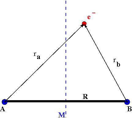
The difficulty in evaluating this integral is a result of the separate spherical coordinate system we use to describe each atom. Thus when we combine the two atoms to make a molecule we end up with three different distances:

• the internuclear separation \(R\) and
• the electron position relative to nucleus \( r_a\)
• the electron position relative to nucleus \( r_b\)

and four angles \(\phi_A\), \(\theta_A\), \(\phi_B\), and \(\theta_B\) two from each nucleus.

Figure \(\PageIndex{1}\): Hydrogen molecular ion \(H^+_2\) with fixed nuclei A and B, internuclear distance R.

There are two ways to address the coordinate system of the overlap integral.

1. Change from two spherical coordinates into one elliptic coordinate system.
2. Use the law of cosines to express \(r_b\) in terms of the coordinates of atom A.

The natural coordinates for a two-center system like \(H_2\) are elliptical and provides the easiest path to evaluating the integral, however many students are not aware of this method because elliptical coordinates are rarely, maybe never, taught in other math and physics classes. Using the law of cosines is a long and arduous integral as it requires trig and u substitution to complete. A step by step guide to method 1 is provided and an outline for how to use method 2.

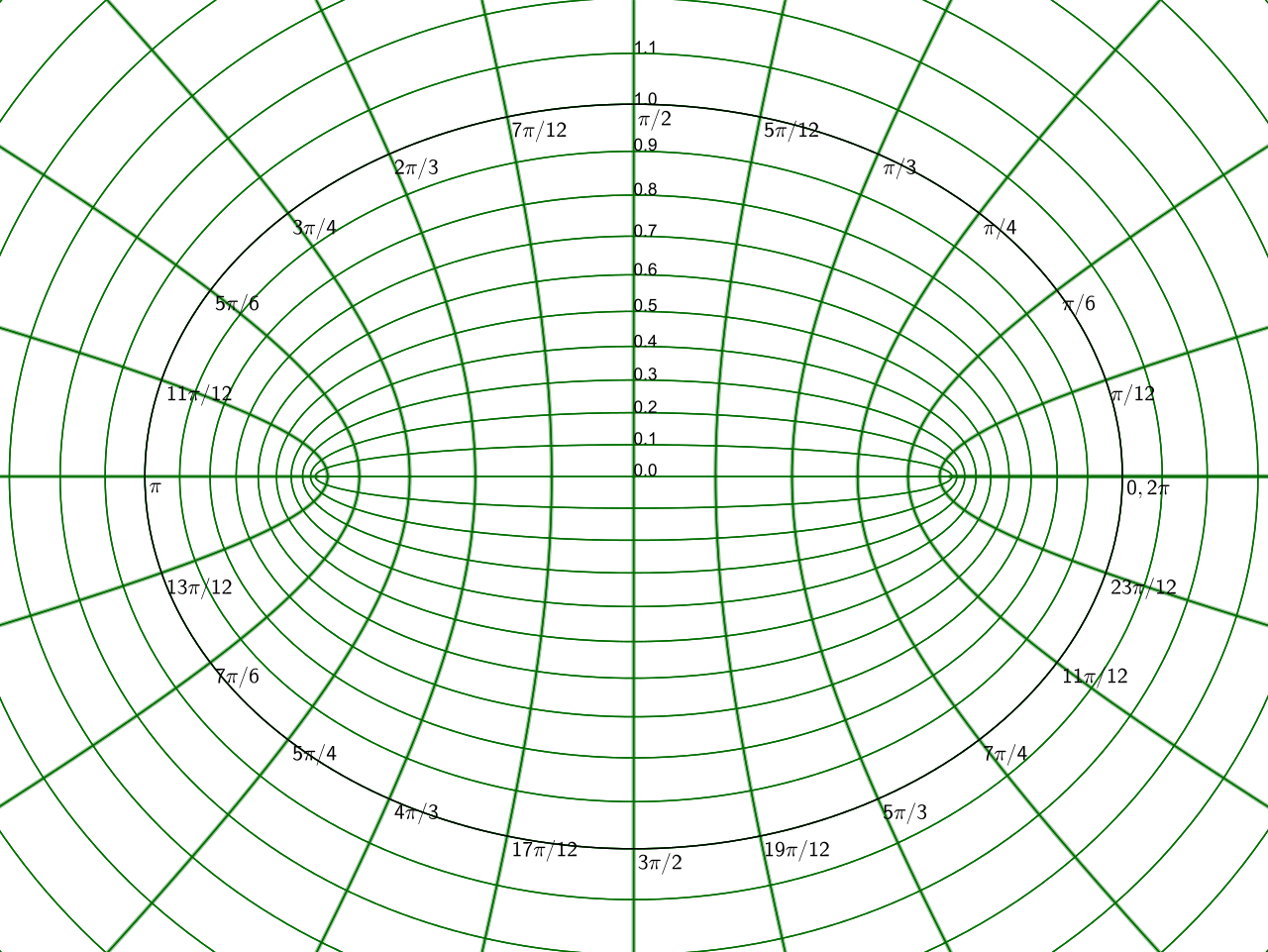
Method 1: Two-Center Elliptical Coordinates

In the two-center elliptical system the any point \(P\) can be expressed by three coordinates \(\lambda, \mu, \phi\) where:

• \(1\leq \lambda < \infty\)
• \(-1 \leq \mu \leq 1 \)
• \(0 \leq \theta \leq 2\pi\)

Figure \(\PageIndex{1}\): Grid for elliptical coordinates. Elliptical grid lines are in even steps of μ of 0.1 units. Hyperbolic grid lines are in even steps of ν of pi/12 for the interval [0,2pi]. a is equal to 1. Image used with permission (GDLF; SharkD).

With this system

\[\lambda = \dfrac{r_a + r_b}{R} \]

\[\mu = \dfrac{r_a - r_b}{R}\]

and the Jacobian or volume element is:

\[d\tau = \dfrac{R^3}{8}(\lambda^2 - \mu^2) d\lambda d\mu d\theta \]

Back to the overlap integral \(S\)

\[S = \int 1s_A 1s_B d\tau\]

The 1s wavefunction is

\[\psi_{100} = \dfrac {1}{\sqrt {\pi}} \left(\dfrac {Z}{a_0}\right)^{\frac {3}{2}} e^{-Zr/a_0}\]

Putting the \(1s_A\) and \(1s_B\) wave functions into the overlap integral still in two sets spherical coordinates we have:

\[S = \int 1s_A 1s_B d\tau\ = \int \dfrac {1}{\sqrt {\pi}} \left(\dfrac {Z}{a_0}\right)^{\frac {3}{2}} e^{-Zr_a/a_0} \times \dfrac {1}{\sqrt {\pi}} \left(\dfrac {Z}{a_0}\right)^{\frac {3}{2}} e^{-Zr_b/a_0} d\tau \]

Still in two sets of spherical coordinates:

\[S = \int 1s_A 1s_B d\tau\ = \dfrac {Z^3}{a_0^3\pi} \int e^{-Zr_a/a_0} e^{-Zr_b/a_0} d \tau \]

\[S = \int 1s_A 1s_B d\tau\ = \dfrac {Z^3}{a_0^3\pi} \int e^{\frac{-Z(r_a + r_b)}{a_0}} d \tau \]

Notice that we only have the \(r_a\) and \(r_b\) coordinates represented. The \(R\) distance in the integral is not present.

Change coordinates:

From our definition above

\[R\lambda = r_a + r_b\]

\[S = \int 1s_A 1s_B d\tau\ = \dfrac {Z^3}{a_0^3\pi} \int e^{\frac{-RZ\lambda}{a_0}} d \tau \]

Look how \(R\) becomes part of the integral naturally when the coordinate system changes. There is no need to convert the spherical angles \(\phi_A\), \(\theta_A\), \(\phi_B\), and \(\theta_B\) into elliptical coordinates because they are not present in the original spherical integral, or in the wavefunctions.

Put in the Jacobian and:

\[S = \int 1s_A 1s_B d\tau\ = \dfrac {Z^3}{a_0^3\pi} \dfrac{R^3}{8} \int_1^{\infty} \int_{-1}^1 \int_0^{2\pi} e^{\frac{-RZ\lambda}{a_0}} (\lambda^2 - \mu^2) d\lambda d\mu d\theta \]

\[S = \int 1s_A 1s_B d\tau\ = \dfrac {Z^3}{a_0^3\pi} \dfrac{R^3}{8} \int_0^{2\pi} d\theta \Big[ \int_1^{\infty} \int_{-1}^1 \lambda^2 e^{\frac{-RZ\lambda}{a_0}} d\lambda d\mu - \int_1^{\infty} \int_{-1}^1 \mu^2 e^{\frac{-RZ\lambda}{a_0}} d\lambda d\mu \Big] \]

Lets simplfy this a little bit by noting that \(Z=1\) for hydrogen and evaluating the angular part.

\[S = \int 1s_A 1s_B d\tau\ = \dfrac {1}{a_0^3} \dfrac{R^3}{4} \Big[ \int_1^{\infty} \int_{-1}^1 \lambda^2 e^{\frac{-R\lambda}{a_0}} d\lambda d\mu - \int_1^{\infty} \int_{-1}^1 \mu^2 e^{\frac{-R\lambda}{a_0}} d\lambda d\mu \Big] \]

Next the \(d\mu\) integrals

\[S = \int 1s_A 1s_B d\tau\ = \dfrac {1}{a_0^3} \dfrac{R^3}{4} \left[ 2 \int_1^{\infty} \lambda^2 e^{\frac{-R\lambda}{a_0}} d\lambda - \dfrac{2}{3} \int_1^{\infty} e^{\frac{-R\lambda}{a_0}} d\lambda \right] \]

To finish we need the excellent integral

\[\int_t^{\infty} z^n e^{-bz} = \dfrac{n!}{b^{n+1}} \left( 1 + bt + \dfrac{b^2t^2}{2!} + .... \dfrac{b^nt^n}{n!} \right) \]

where \(n = 0,1,2,3,4,... \) and \(b>0\)

In our case \(n = 0 \) and \(2\) with \(t = 1\) and \(b = R/a_0\)

\[S = \int 1s_A 1s_B d\tau\ = \dfrac {1}{a_0^3} \dfrac{R^3}{4} \left[ 2 \dfrac{2a_0^3}{R^3} e^{-R/a_0}\left(1 + \dfrac{R}{a_0} + \dfrac{R^2}{2a^2_0} \right) - \dfrac{2}{3} \dfrac{a_0}{R} e^{-R/a_0} \left( 1 \right) \right] \]

Distribute the constant out front

\[S = \int 1s_A 1s_B d\tau\ = \left[ e^{-R/a_0} \left(1 + \dfrac{R}{a_0} + \dfrac{R^2}{2a^2_0} \right) - \dfrac {R^2}{6a_0^2} e^{-R/a_0} \right] \]

Pull out the exponent and ....

\[S = \int 1s_A 1s_B d\tau\ = e^{-R/a_0}\left[ 1 + \dfrac{R}{a_0} + \dfrac{R^2}{2a^2_0} - \dfrac {R^2}{6a_0^2} \right] \]

The Answer -

\[S(R) = \int 1s_A 1s_B d\tau\ = e^{-R/a_0}\left[ 1 + \dfrac{R}{a_0} + \dfrac{R^2}{3a^2_0} \right] \]

Method 2: The Law of Cosines

Work in Progress...

References

• http://www.colby.edu/chemistry/PChem...structions.pd
• Recursion formulae for calculation of overlap integrals, January 1987. 10.1002/jcc.540080102
• Formulas and Numerical Tables for Overlap Integrals R. S. Mulliken, C. A. Rieke, D. Orloff and H. Orloff, J. Chem. Phys. 17, 1248 (1949); http://dx.doi.org/10.1063/1.1747150