16: Linear Momentum and Electronic Spectroscopy

Recap of Lecture 15

Last lecture continued the discussion of the 3D rigid rotor. We discussed the three aspect of the solutions to this system: The wavefunctions (the spherical harmonics), the energies (and degeneracies) and the TWO quantum numbers (\(J\) and \(m_J\)) and their ranges. We discussed that the components of the angular momentum operator are subject to the Heisenberg uncertainty principle and cannot be known to infinite precision simultaneously, however the magnitude of angular momentum and any component can be. This results in the vectoral representation of angular momentum

Spherical Harmonics in Rigid Rotors

The wavefunction of a rigid rotor can be separte (via the separation of variables approach) into product of two functions:

\[ \color{red} | Y(\theta, \phi) \rangle = |\Theta(\theta) \rangle| \Phi(\phi) \rangle\]

The \(\Phi\) function is found to have quantum number \(m\). \(\Phi_m (\phi) = A_m e^{im\phi}\), where \(A_m\) is the normalization constant and \(m = 0, \pm1, \pm2 ... \pm\infty\). The \(\Theta\) function was solved and is known as Legendre polynomials, which have quantum numbers \(m\) and \(\ell\). When \(\Theta\) and \(\Phi\) are multiplied together, the product is known as spherical harmonics with labeling \(Y_{J}^{m} (\theta, \phi)\).

\(m_J\)	\(J\)	\(\Theta ^{m_J}_J (\theta)\)	\(\Phi (\varphi)\)	\(Y^{m_J}_J (\theta , \varphi)\)
0	0	\(\dfrac {1}{\sqrt {2}}\)	\(\dfrac {1}{\sqrt {2 \pi}}\)	\(\dfrac {1}{\sqrt {4 \pi}}\)
0	1	\(\sqrt {\dfrac {3}{2}}\cos \theta\)	\(\dfrac {1}{\sqrt {2 \pi}}\)	\(\sqrt {\dfrac {3}{4 \pi}}\cos \theta\)
1	1	\(\sqrt {\dfrac {3}{4}}\sin \theta\)	\(\dfrac {1}{\sqrt {2 \pi}}e^{i \varphi}\)	\(\sqrt {\dfrac {3}{8 \pi}}\sin \theta e^{i \varphi}\)
-1	1	\(\sqrt {\dfrac {3}{4}}\sin \theta\)	\(\dfrac {1}{\sqrt {2 \pi}}e^{-i\varphi}\)	\(\sqrt {\dfrac {3}{8 \pi}}\sin \theta e^{-i \varphi}\)
0	2	\(\sqrt {\dfrac {5}{8}}(3\cos ^2 \theta - 1)\)	\(\dfrac {1}{\sqrt {2 \pi}}\)	\(\sqrt {\dfrac {5}{16\pi}}(3\cos ^2 \theta - 1)\)
1	2	\(\sqrt {\dfrac {15}{4}} \sin \theta \cos \theta \)	\(\dfrac {1}{\sqrt {2 \pi}}e^{i \varphi}\)	\(\sqrt {\dfrac {15}{8\pi}} \sin \theta \cos \theta e^{i\varphi}\)
-1	2	\(\sqrt {\dfrac {15}{4}} \sin \theta \cos \theta \)	\(\dfrac {1}{\sqrt {2 \pi}}e^{-i\varphi}\)	\(\sqrt {\dfrac {15}{8\pi}} \sin \theta \cos \theta e^{-i\varphi}\)
2	2	\(\sqrt {\dfrac {15}{16}} \sin ^2 \theta \)	\(\dfrac {1}{\sqrt {2 \pi}}e^{2i\varphi}\)	\(\sqrt {\dfrac {15}{32\pi}} \sin ^2 \theta e^{2i\varphi} \)
-2	2	\(\sqrt {\dfrac {15}{16}} \sin ^2 \theta \)	\(\dfrac {1}{\sqrt {2 \pi}}e^{2i\varphi}\)	\(\sqrt {\dfrac {15}{32\pi}} \sin ^2 \theta e^{-2i\varphi} \)

Figure used with permission (CC-SA-BY- 3.0; Sarxos)

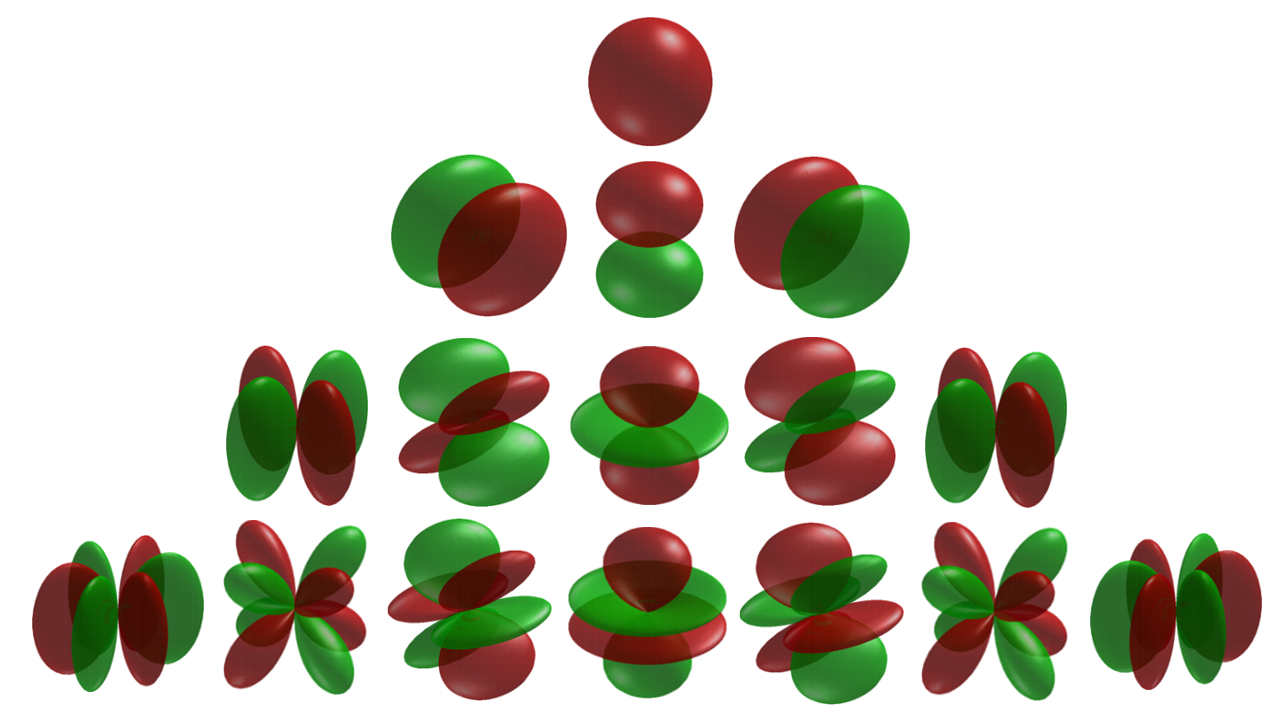
The above figure show the spherical harmonics \(Y_J^M\), which are solutions of the angular Schrödinger equation of a 3D rigid rotor.

Microwave Spectroscopy Probes Rotations

The permanent electric dipole moments of polar molecules can couple to the electric field of electromagnetic radiation. This coupling induces transitions between the rotational states of the molecules. The energies that are associated with these transitions are detected in the far infrared and microwave regions of the spectrum. For example, the microwave spectrum for carbon monoxide spans a frequency range of 100 to 1200 GHz, which corresponds to 3 - 40 \(cm^{-1}\).

The selection rules for the rotational transitions are derived from the transition moment integral by using the spherical harmonic functions and the appropriate dipole moment operator, \(\hat {\mu}\).

\[ \mu _T = \int Y_{J_f}^{m_f*} \hat {\mu} Y_{J_i}^{m_i} \sin \theta \,d \theta \,d \varphi \label {5.9.1} \]

Evaluating the transition moment integral involves a bit of mathematical effort. This evaluation reveals that the transition moment depends on the square of the dipole moment of the molecule, \(\mu ^2\) and the rotational quantum number, \(J\), of the initial state in the transition,

\[\mu _T = \mu ^2 \dfrac {J + 1}{2J + 1} \label {5.9.2}\]

and that the selection rules for rotational transitions are

\[ \color{red} \Delta J = \pm 1 \label {5.9.3}\]

\[ \color{red} \Delta m_J = 0, \pm 1 \label {5.9.4}\]

A photon is absorbed for \(\Delta J = +1\) and a photon is emitted for \(\Delta J = -1\).

The energies of the rotational levels are given by

\[E = J(J + 1) \dfrac {\hbar ^2}{2I} \]

and each energy level has a degeneracy of \(2J+1\) due to the different \(m_J\) values.

Each energy level of a rigid rotor has a degeneracy of \(2J+l\) due to the different \(m_J\) values.

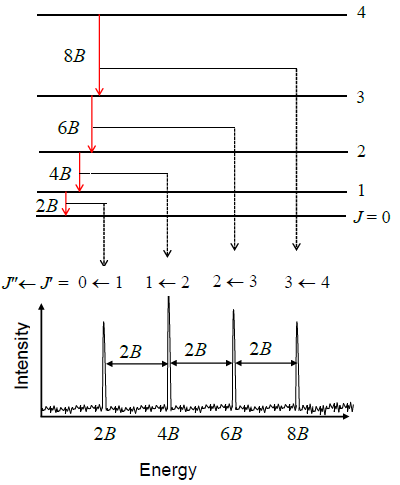
The transition energies for absorption of radiation are given by

\[\Delta E_{states} = E_f - E_i = E_{photon} = h \nu = hc \bar {\nu} \label {5.9.5}\]

\[h \nu =hc \bar {\nu} = J_f (J_f +1) \dfrac {\hbar ^2}{2I} - J_i (J_i +1) \dfrac {\hbar ^2}{2I} \label {5.9.6}\]

Since microwave spectroscopists use frequency, and infrared spectroscopists use wavenumber units when describing rotational spectra and energy levels, both \(\nu\) and \(\bar {\nu}\) are included in Equation \(\ref{5.9.6}\), and \(J_i\) and \(J_f\) are the rotational quantum numbers of the initial (lower) and final (upper) levels involved in the absorption transition. When we add in the constraints imposed by the selection rules, \(J_f\) is replaced by \(J_i + 1\), because the selection rule requires \(J_f – J_i = 1\) for absorption. The equation for absorption transitions then can be written in terms of the quantum number \(J_i\) of the initial level alone.

\[h \nu = hc \bar {\nu} = 2 (J_i + 1) \dfrac {\hbar ^2}{2I} \label {5.9.7}\]

Divide Equation \(\ref{5.9.7}\) by \(h\) to obtain the frequency of the allowed transitions,

\[ \nu = 2B (J_i + 1) \label {5.9.8}\]

where \(B\), the rotational constant for the molecule, is defined as

\[B = \dfrac{h}{8\pi^2 I}\]

or in terms of wavenumber

\[\tilde{B} = \dfrac{h}{8\pi^2 c I} \label {5.9.9}\]

The rotation spectrum of \(^{12}C^{16}O\) at 40 K.

This microwave spectrum can be decomposed into eigenstates thusly

Energy levels and line positions calculated in the rigid rotor approximation. (CC BY-SA 3.0 unported; Nnrw via Wikipedia)

The rotational constant is quite sensitive to the geometry of the molecule and can be big for molecules that have small moments of inertia (i.e., like \(\ce{H2}\)) or small for molecules that have large moments of inertia (i.e., \(\ce{I2}\)) as expected from reviewing Equation \ref{5.9.9}.

Equilibrium distances and rotational and vibrational constants in units of cm−1 for some diatomic molecules

Molecule	\(\ce{H2}\)	\(\ce{Li2}\)	\(\ce{N2}\)	\(\ce{O2}\)	\(\ce{I2}\)	\(\ce{H^{35}Cl}\)	\(\ce{D^{35}Cl}\)
\(\tilde{B}\)	60.8	0.673	2.01	1.45	0.0037	10.59	5.45

Example \(\PageIndex{1}\): Carbon Monoxide

Calculate the bondlength of carbon monoxide if the \(J = 0\) to \(J = 1\) transition for \(^{12}C^{16}O\) in its microwave spectrum is \(1.153 \times 10^{5} MHz\).

Solution:

Assuming that \(^{12}C^{16}O\) can be treated as a ridged rotor

\[\nu = 2B(J + 1)\]

with \(J = 1, 2, 3, . . .\) and \(B = \dfrac{h}{8\pi^2l}\)

For the \(J = 0\) to \(J = 1\) transition,

\[\dfrac {1}{2}\nu = B = \dfrac{h}{8\pi^2l}\]

\[\dfrac {1}{2}1.153 \times 10^{11} s^{-1} = B = \dfrac{6.626 \times 10^{-34} J.s}{8\pi^2\mu r^2}\]

We can find \(\mu\) and use the relationship \(r^2 = \dfrac{1}{\mu}\) to find \(r\).

\[\mu = \dfrac{(12.00)(15.99)}{27.99} 1.661 \times 10^{-27} kg = 1.139 \times 10^{-26} kg\]

\[r^2 = \dfrac{6.626 \times 10^{-34} J.s}{4pi^2 1.139 \times 10^{-26} kg 1.153 \times 10^{11} s^-1}\]

= \(1.13 \times 10^{-10} m\) = 113 pm

Thus the bondlength in carbon monoxide is 113 pm.

Contributors

• Richard Fitzpatrick (Professor of Physics, The University of Texas at Austin)