
11: Postulate of Quantum Mechanics (Lecture)
- Page ID
- 198576

\( \newcommand{\vecs}[1]{\overset { \scriptstyle \rightharpoonup} {\mathbf{#1}} } \)
\( \newcommand{\vecd}[1]{\overset{-\!-\!\rightharpoonup}{\vphantom{a}\smash {#1}}} \)
\( \newcommand{\id}{\mathrm{id}}\) \( \newcommand{\Span}{\mathrm{span}}\)
( \newcommand{\kernel}{\mathrm{null}\,}\) \( \newcommand{\range}{\mathrm{range}\,}\)
\( \newcommand{\RealPart}{\mathrm{Re}}\) \( \newcommand{\ImaginaryPart}{\mathrm{Im}}\)
\( \newcommand{\Argument}{\mathrm{Arg}}\) \( \newcommand{\norm}[1]{\| #1 \|}\)
\( \newcommand{\inner}[2]{\langle #1, #2 \rangle}\)
\( \newcommand{\Span}{\mathrm{span}}\)
\( \newcommand{\id}{\mathrm{id}}\)
\( \newcommand{\Span}{\mathrm{span}}\)
\( \newcommand{\kernel}{\mathrm{null}\,}\)
\( \newcommand{\range}{\mathrm{range}\,}\)
\( \newcommand{\RealPart}{\mathrm{Re}}\)
\( \newcommand{\ImaginaryPart}{\mathrm{Im}}\)
\( \newcommand{\Argument}{\mathrm{Arg}}\)
\( \newcommand{\norm}[1]{\| #1 \|}\)
\( \newcommand{\inner}[2]{\langle #1, #2 \rangle}\)
\( \newcommand{\Span}{\mathrm{span}}\) \( \newcommand{\AA}{\unicode[.8,0]{x212B}}\)
\( \newcommand{\vectorA}[1]{\vec{#1}} % arrow\)
\( \newcommand{\vectorAt}[1]{\vec{\text{#1}}} % arrow\)
\( \newcommand{\vectorB}[1]{\overset { \scriptstyle \rightharpoonup} {\mathbf{#1}} } \)
\( \newcommand{\vectorC}[1]{\textbf{#1}} \)
\( \newcommand{\vectorD}[1]{\overrightarrow{#1}} \)
\( \newcommand{\vectorDt}[1]{\overrightarrow{\text{#1}}} \)
\( \newcommand{\vectE}[1]{\overset{-\!-\!\rightharpoonup}{\vphantom{a}\smash{\mathbf {#1}}}} \)
\( \newcommand{\vecs}[1]{\overset { \scriptstyle \rightharpoonup} {\mathbf{#1}} } \)
\( \newcommand{\vecd}[1]{\overset{-\!-\!\rightharpoonup}{\vphantom{a}\smash {#1}}} \)
\(\newcommand{\avec}{\mathbf a}\) \(\newcommand{\bvec}{\mathbf b}\) \(\newcommand{\cvec}{\mathbf c}\) \(\newcommand{\dvec}{\mathbf d}\) \(\newcommand{\dtil}{\widetilde{\mathbf d}}\) \(\newcommand{\evec}{\mathbf e}\) \(\newcommand{\fvec}{\mathbf f}\) \(\newcommand{\nvec}{\mathbf n}\) \(\newcommand{\pvec}{\mathbf p}\) \(\newcommand{\qvec}{\mathbf q}\) \(\newcommand{\svec}{\mathbf s}\) \(\newcommand{\tvec}{\mathbf t}\) \(\newcommand{\uvec}{\mathbf u}\) \(\newcommand{\vvec}{\mathbf v}\) \(\newcommand{\wvec}{\mathbf w}\) \(\newcommand{\xvec}{\mathbf x}\) \(\newcommand{\yvec}{\mathbf y}\) \(\newcommand{\zvec}{\mathbf z}\) \(\newcommand{\rvec}{\mathbf r}\) \(\newcommand{\mvec}{\mathbf m}\) \(\newcommand{\zerovec}{\mathbf 0}\) \(\newcommand{\onevec}{\mathbf 1}\) \(\newcommand{\real}{\mathbb R}\) \(\newcommand{\twovec}[2]{\left[\begin{array}{r}#1 \\ #2 \end{array}\right]}\) \(\newcommand{\ctwovec}[2]{\left[\begin{array}{c}#1 \\ #2 \end{array}\right]}\) \(\newcommand{\threevec}[3]{\left[\begin{array}{r}#1 \\ #2 \\ #3 \end{array}\right]}\) \(\newcommand{\cthreevec}[3]{\left[\begin{array}{c}#1 \\ #2 \\ #3 \end{array}\right]}\) \(\newcommand{\fourvec}[4]{\left[\begin{array}{r}#1 \\ #2 \\ #3 \\ #4 \end{array}\right]}\) \(\newcommand{\cfourvec}[4]{\left[\begin{array}{c}#1 \\ #2 \\ #3 \\ #4 \end{array}\right]}\) \(\newcommand{\fivevec}[5]{\left[\begin{array}{r}#1 \\ #2 \\ #3 \\ #4 \\ #5 \\ \end{array}\right]}\) \(\newcommand{\cfivevec}[5]{\left[\begin{array}{c}#1 \\ #2 \\ #3 \\ #4 \\ #5 \\ \end{array}\right]}\) \(\newcommand{\mattwo}[4]{\left[\begin{array}{rr}#1 \amp #2 \\ #3 \amp #4 \\ \end{array}\right]}\) \(\newcommand{\laspan}[1]{\text{Span}\{#1\}}\) \(\newcommand{\bcal}{\cal B}\) \(\newcommand{\ccal}{\cal C}\) \(\newcommand{\scal}{\cal S}\) \(\newcommand{\wcal}{\cal W}\) \(\newcommand{\ecal}{\cal E}\) \(\newcommand{\coords}[2]{\left\{#1\right\}_{#2}}\) \(\newcommand{\gray}[1]{\color{gray}{#1}}\) \(\newcommand{\lgray}[1]{\color{lightgray}{#1}}\) \(\newcommand{\rank}{\operatorname{rank}}\) \(\newcommand{\row}{\text{Row}}\) \(\newcommand{\col}{\text{Col}}\) \(\renewcommand{\row}{\text{Row}}\) \(\newcommand{\nul}{\text{Nul}}\) \(\newcommand{\var}{\text{Var}}\) \(\newcommand{\corr}{\text{corr}}\) \(\newcommand{\len}[1]{\left|#1\right|}\) \(\newcommand{\bbar}{\overline{\bvec}}\) \(\newcommand{\bhat}{\widehat{\bvec}}\) \(\newcommand{\bperp}{\bvec^\perp}\) \(\newcommand{\xhat}{\widehat{\xvec}}\) \(\newcommand{\vhat}{\widehat{\vvec}}\) \(\newcommand{\uhat}{\widehat{\uvec}}\) \(\newcommand{\what}{\widehat{\wvec}}\) \(\newcommand{\Sighat}{\widehat{\Sigma}}\) \(\newcommand{\lt}{<}\) \(\newcommand{\gt}{>}\) \(\newcommand{\amp}{&}\) \(\definecolor{fillinmathshade}{gray}{0.9}\)Recap of Lecture 10: Expectation values, 2D-PIB and Heisenberg Uncertainty Principle
Last lecture focused on the extension of the 1D particle in a box to the 2-D and 3D cases. This is an easy problem since via a simple application of separation of variables (Worksheet 2) for each dimension (they act independently). From this we identified a few interesting phenomena including multiple quantum numbers (\(n_x\), \(n_y\) and \(n_z\)) and degeneracy (if the boxes are of the same length or multiples of each other) where multiple wavefunctions share the identical energy.
We were able to provide a quantitative backing in using the Heisenberg Uncertainty principle from wavefuctions, specifically in terms of the standard deviations of the probability distribution functions (i.e., wavefunction squared).
We ended the lecture on the five postulates of quantum mechanics, which ties together many aspects that we have been discussing.
3D Boxes Redux
The 1D particle in the box problem can be expanded to consider a particle within a 3D box for three lengths \(a\), \(b\), and \(c\). When there is NO FORCE (i.e., no potential) acting on the particles inside the box.
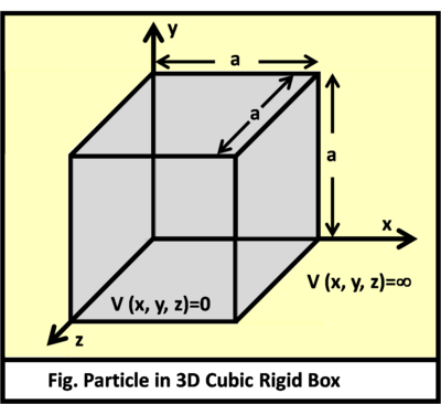
The potential for the particle inside the box
\[V(\vec{r}) = 0\]
- \(0 \leq x \leq a\)
- \(0 \leq y \leq b\)
- \(0 \leq z \leq c\)
- \(a < x < 0\)
- \(b < y < 0\)
- \(c < z < 0\)
\(\vec{r}\) is the vector with all 3 components along the 3 axis of the 3-D box: \(\vec{r} = a\hat{x} + b\hat{y} + c\hat{z}\). When the potential energy is infinite, then the wave function equals zero. When the potential energy is zero, then the wavefunction obeys the Schrödinger equation.
\[\psi(r) = \sqrt{\dfrac{8}{v}}\sin \left( \dfrac{n_{x} \pi x}{a} \right) \sin \left(\dfrac{n_{y} \pi y}{b}\right) \sin \left(\dfrac{ n_{z} \pi z}{c} \right)\]
\[v = a \times b \times c = volume \; of \; box\]
with Total Energy levels:
\[E_{n_x,n_y,x_z} = \dfrac{h^{2}}{8m}\left(\dfrac{n_{x}^{2}}{a^{2}} + \dfrac{n_{y}^{2}}{b^{2}} + \dfrac{n_{z}^{2}}{c^{2}}\right) \label{3.9.10}\]
As with 1-D boxes, the quantum numbers \(n_x\), \(n_y\), and \(n_z\) go from 1 to infinity.
Exercise \(\PageIndex{1}\)
What is the energy of the ground state of a 3D box that is \(a\) by \(a\) by \(a\)?
- Answer:
-
This is when \(n_x=1\), \(n_y=1\), and \(n_z=1\). So from Equation \(\ref{3.9.10}\), this is
\[E_{1,1,1}= \dfrac{h^{2}}{8m}\left(\dfrac{1}{a^{2}} + \dfrac{1}{a^{2}} + \dfrac{1}{a^{2}}\right) = \dfrac{3h^{2}}{8ma^{2}} \]
Exercise \(\PageIndex{2}\)
What is the energy of the 1st excited state of a 3D box that is \(a\) by \(a\) by \(a\)?
- Answer:
-
This is trickier, since there is a degeneracy in the system with three wavefunctions having the same energy:
- \(\Psi_{2,1,1}\)
- \(\Psi_{1,2,1}\)
- \(\Psi_{1,1,2}\)
Each of these wavefunctions have the same energy (via Equation \(\ref{3.9.10}\)) of
\[E= \dfrac{6h^{2}}{8ma^{2}}\]
Postulates of Quantum Mechanics in a Nutshell (you know all these already)
There are five assumptions made for the purpose of reasoning in quantum mechanics. These assumptions are called postulates, and they set the groundwork for quantum mechanics.
Postulate 1
The state of the system is completely specified by \(\psi\). All possible information about the system can be found in the wavefunction \(\psi\). For valid, well-behaved wavefunctions, normalized probability holds true, such that the integral over all space is equal to 1.
\[\int_{-\infty}^\infty \psi^*(x)\psi(x)\;dx=1.\]
What this means is that the chance to find a particle is 100% over all space. Wavefunctions must be- single valued,
- continuous, and
- finite.
Postulate 2
For every observable in classical mechanics, there is a corresponding operator in quantum mechanics.| Name | Observable Symbol | Operator Symbol | Operation |
|---|---|---|---|
| Position | \(x\) | \(\hat{X}\) | Multiply by \(x\) |
| \(r\) | \(\hat{R}\) | Multiply by \(r\) | |
| Momentum | \(p_{x}\) | \(\hat{P_{x}}\) | -\(\imath \hbar \dfrac{d}{dx}\) |
| \(p\) | \(\hat{P}\) | -\(\imath\)\(\hbar\)[\(\text{i}\)\(\dfrac{d}{dx}\)+\(\text{j}\)\(\dfrac{d}{dy}\)+\(\text{k}\)\(\dfrac{d}{dz}\)] | |
| Kinetic Energy | \(K_{x}\) | \(\hat{K_{x}}\) | \(\dfrac{-(\hbar^{2})}{2m}\)\(\dfrac{d^{2}}{dx^{2}}\) |
| \(K\) | \(\hat{K}\) |
\(\dfrac{-(\hbar^{2})}{2m}\)[\(\dfrac{d^{2}}{dx^{2}}\)+\(\dfrac{d^{2}}{dy^{2}}\)+\(\dfrac{d^{2}}{dz^{2}}\)] Which can be simplified to |
|
| Potential Energy | \(V(x)\) | \(\hat{V(x)}\) | Multiply by \(V(x)\) |
| \(V(x,y,z)\) | \(\hat{V(x,y,z)}\) | Multiply by \(V(x,y,z)\) | |
| Total Energy | \(E\) | \(\hat{E}\) | \(\dfrac{-(\hbar^{2})}{2m}\)\(\bigtriangledown^{2}\) + \(V(x,y,z)\) |
| Angular Momentum | \(L_{x}\) | \(\hat{L_{x}}\) | -\(\imath\)\(\hbar\)[\(\text{y}\)\(\dfrac{d}{dz}\) - \(\text{z}\)\(\dfrac{d}{dy}\)] |
| \(L_{y}\) | \(\hat{L_{y}}\) | -\(\imath\)\(\hbar\)[\(\text{z}\)\(\dfrac{d}{dx}\) - \(\text{x}\)\(\dfrac{d}{dz}\)] | |
| \(L_{z}\) | \(\hat{L_{z}}\) | -\(\imath\)\(\hbar\)[\(\text{x}\)\(\dfrac{d}{dy}\) - \(\text{y}\)\(\dfrac{d}{dx}\)] |
Postulate 3
If \(\hat{A}\)\(\psi(x)\) produces eigenvalues \(\{a\}\), where
\[\hat{A} \psi_n(x) = a_n \psi_n(x)\]
then the set \(\{a_n\}\) is the set of values (and only those values) that can be observed.
Postulate 4
For a normalized wavefunction, the average value of any observable with operation \(\hat{A}\) is given by
\[\langle a \rangle = \int_{-\infty}^\infty \psi^*(x) \hat{A}\ \psi(x) dx\]
Postulate 5
Wavefunctions evolve in time, given by the Time-dependent Schrödinger Equation
\[\hat{H}\Psi(x,t) = \imath \hbar \dfrac{d(\Psi(x,t))}{dt}\]
where
\[\Psi(x,t) = \psi(x)f(t)\]
Using the Separation of Variables technique results in
\[f(t)= e^\frac {-iEt}{\hbar} = e^{-it\omega}\]
Commuting Operators
One important property of operators is that the order of operation matters. Thus:
\[\hat{A}{\hat{E}f(x)} \not= \hat{E}{\hat{A}f(x)} \label{4.6.3}\]
unless the two operators commute. Two operators commute if the following equation is true:
\[\left[\hat{A},\hat{E}\right] = \hat{A}\hat{E} - \hat{E}\hat{A} = 0 \label{4.6.4}\]
To determine whether two operators commute first operate \(\hat{A}\hat{E}\) on a function \(f(x)\). Then operate\(\hat{E}\hat{A}\) the same function \(f(x)\). If the same answer is obtained subtracting the two functions will equal zero and the two operators will commute.
Example \(\PageIndex{1}\)
Do \(\hat{A}\) and \(\hat{E} \) commute if
\[\hat{A} = \dfrac{d}{dx}\]
and
\[\hat{E} = x^2\]
- Solution
-
This requires evaluating \(\left[\hat{A},\hat{E}\right]\), which requires solving for \(\hat{A} \{\hat{E} f(x)\} \) and \(\hat{E} \{\hat{A} f(x)\}\) for arbitrary wavefunction \(f(x)\) and asking if they are equal.
\[\hat{A} \{\hat{E} f(x)\} = \hat{A}\{ x^2 f(x) \}= \dfrac{d}{dx} \{ x^2 f(x)\} = 2xf(x) + x^2 f'(x)\]
From the product rule of differentiation.
\[\hat{E} \{\hat{A}f(x)\} = \hat{E}\{f'(x)\} = x^2 f'(x)\]
Now ask if they are equal
\[\left[\hat{A},\hat{E}\right] = 2x f(x) + x^2 f'(x) - x^2f'(x) = 2x f(x) \not= 0\]
Therefore the two operators do not commute.
Example \(\PageIndex{2}\)
Do \(\hat{B}\) and \(\hat{C} \) commute if
\[\hat{B}= \dfrac {h} {x}\]
and
\[\hat{C}\{f(x)\} = f(x) +3\]
- Solution
- This requires evaluating \(\left[\hat{B},\hat{C}\right]\) like in Example \(\PageIndex{1}\).
\[\hat{B} \{\hat{C}f(x)\} = \hat{B}\{f(x) +3\} = \dfrac {h}{x} (f(x) +3) = \dfrac {h f(x)}{x} + \dfrac{3h}{x} \]
\[\hat{C} \{\hat{B}f(x)\} = \hat{C} \{ \dfrac {h} {x} f(x)\} = \dfrac {h f(x)} {x} +3\]
Now ask if they are equal
\(\left[\hat{B},\hat{C}\right] = \dfrac {h f(x)} {x} + \dfrac {3h} {x} - \dfrac {h f(x)} {x} -3 \not= 0\)
The two operators do not commute.
Heisenberg Uncertainty Principle Redux (Redux Redux)
Although it will not be proven here, there is a general statement of the uncertainty principle in terms of the commutation property of operators. If two operators \(\hat {A}\) and \(\hat {B}\) do not commute, then the uncertainties (standard deviations σ) in the physical quantities associated with these operators must satisfy
\[\sigma _A \sigma _B \ge \left| \int \psi ^* [ \hat {A} \hat {B} - \hat {B} \hat {A} ] \psi d\tau \right| \label{4-52}\]
where the integral inside the square brackets is called the commutator, and ││signifies the modulus or absolute value. If \(\hat {A}\) and \(\hat {B}\) commute, then the right-hand-side of equation \(\ref{4-52}\) is zero, so either or both \(σ_A\) and \(σ_B\) could be zero, and there is no restriction on the uncertainties in the measurements of the eigenvalues \(a\) and \(b\).